Discrete harmonic function

旧博客原文

原题：Discrete harmonic function in Z^n

There is some gap, in fact I can improve half of the argument of Discrete harmonic function , the pdf version is Discrete harmonic function in Z^n, but I still have some gap to deal with the residue half…

1. The statement of result

First of all, we give the definition of discrete harmonic function.

Definition 1 (Discrete harmonic function) We say a function ${f: {\mathbb Z}^n \rightarrow {\mathbb R}}$ is a discrete harmonic function on ${{\mathbb Z}^n}$ if and only if for any ${(x_1,...,x_n)\in {\mathbb Z}^n}$ , we have:

$\displaystyle f(x_1,...,x_n)=\frac{1}{2^n}\sum_{(\delta_1,...,\delta_n )\in \{-1,1\}^n}f(x_1+\delta_1,...,x_n+\delta_n ) \ \ \ \ \ (1)$

In dimension 2, the definition reduce to:

Definition 2 (Discrete harmonic function in ${{\mathbb R}^2}$ ) We say a function ${f: {\mathbb Z}^2 \rightarrow {\mathbb R}}$ is a discrete harmonic function on ${{\mathbb Z}^2}$ if and only if for any ${(x_1,x_2)\in {\mathbb Z}^2}$ , we have:

$\displaystyle f(x_1,x_2)=\frac{1}{4}\sum_{(\delta_1,\delta_2)\in \{-1,1\}^2}f(x_1+\delta_1,x_2+\delta_2 ) \ \ \ \ \ (2)$

The result establish in \cite{paper} is following:

Theorem 3 (Liouville theorem for discrete harmonic functions in ${{\mathbb R}^2}$ ) Given ${c>0}$ . There exists a constant ${\epsilon>0}$ related to ${c}$ such that, given a discrete harmonic function ${f}$ in ${{\mathbb Z}^2}$ satisfied for any ball ${B_R(x_0)}$ with radius ${R>R_0}$ , there is ${1-\epsilon}$ portion of points ${x\in B_R(x_0)}$ satisfied ${|f(x)|<c}$ . then ${f}$ is a constant function in ${{\mathbb Z}^2}$ .

Remark 1 This type of result contradict to the intuition, at least there is no such result in ${{\mathbb C}}$ . For example. the existence of poisson kernel and the example given in \cite{paper} explain the issue.

Remark 2 There are reasons to explain why there could not have a result in ${{\mathbb C}}$ but in ${{\mathbb Z}^2}$ ,

The first reason is due to every radius ${R}$ there is only ${O(R^2)}$ lattices in ${B_R(x)}$ in ${{\mathbb Z}^2}$ so the mass could not concentrate very much in this setting.

The second one is due to there do not have infinite scale in ${{\mathbb Z}^2}$ but in ${{\mathbb C}}$ .

The third one is the function in ${{\mathbb Z}^2}$ is automatically locally integrable.

The generation is following:

Theorem 4 (Liouville theorem for discrete harmonic functions in ${{\mathbb R}^n}$ ) Given ${c>0,n\in {\mathbb N}}$ . There exists a constant ${\epsilon>0}$ related to ${n,c}$ such that, given a discrete harmonic function ${f}$ in ${{\mathbb Z}^n}$ satisfied for any ball ${B_R(x_0)}$ with radius ${R>R_0}$ , there is ${1-\epsilon}$ portion of points ${x\in B_R(x_0)}$ satisfied ${|f(x)|<c}$ . then ${f}$ is a constant function in ${{\mathbb Z}^n}$ .

In this note, I give a proof of 4, and explicit calculate a constant ${\epsilon_n>0}$ satisfied the condition in 3, this way could also calculate a constant ${\epsilon_n}$ satisfied 4. and point the constant calculate in this way is not optimal both in high dimension and 2 dimension.

2. some element properties with discrete harmonic function

We warm up with some naive property with discrete harmonic function. The behaviour of bad points could be controlled, just by isoperimetric inequality and maximum principle we have following result.

Definition 5 (Bad points) We divide points of ${{\mathbb Z}^n}$ into good part and bad part, good part ${I}$ is combine by all point ${x}$ such that ${|f(x)|<c}$ , and ${J}$ is the residue one. So ${A\amalg B={\mathbb Z}^n}$ .

For all ${B_R(0)}$ , we define ${J_R:=J\cap B_R(0), I_R=I\cap B_R(0)}$ for convenient.

Theorem 6 (The distribution of bad points) For all bad points ${J_R}$ in ${B_R(0)}$ , they will divide into several connected part, i.e.

$\displaystyle J_R=\amalg_{i\in S_R}A_i \ \ \ \ \ (3)$

and every part ${A_i}$ satisfied ${A_i\cap \partial B_R(0)\neq \emptyset}$ .

Remark 3 We say ${A}$ is connected in ${{\mathbb Z}^n}$ iff there is a path in ${A}$ connected ${x\rightarrow y, \forall x,y\in A}$ .

Remark 4 the meaning that every point So the behaviour of bad points are just like a tree structure given in the gragh.

Proof: A very naive observation is that for all ${\Omega\subset {\mathbb Z}^n}$ is a connected compact domain, then there is a function

$\displaystyle \lambda_{\Omega}: \partial \longrightarrow {\mathbb R} \ \ \ \ \ (4)$

such that ${\lambda_{\Omega}(x,y)\geq 0, \forall (x,y)\in \Omega \times \mathring{\Omega}}$ . And we have:

$\displaystyle f(x)=\sum_{y\in\partial \Omega}\lambda_{\Omega}(x,y)(y) \ \ \ \ \ (5)$

This could be proved by induction on the diameter if ${\Omega}$ . Then, if there is a connected component of ${\Omega}$ such that contradict to theorem 6 for simplify assume the connected component is just ${\Omega}$ , then use the formula 5we know

$\displaystyle \begin{array}{rcl} \sup_{x\in \Omega}|f(x)| & = & \sup_{x\in \Omega}\sum_{y\in\partial \Omega}\lambda_{\Omega}(x,y)(y) \\ & \leq & \sup_{\partial \Omega}|f(x)| \\ & \leq & c \end{array}$

The last line is due to consider around ${\partial \Omega}$ . But this lead to: ${\forall x\in \Omega, |f(x)|<c}$ which is contradict to the definition of ${\Omega}$ . So we get the proof. $\Box$

Now we begin another observation, that is the freedom of extension of discrete harmonic function in ${{\mathbb Z}^n}$ is limited.

Theorem 7 we can say something about the structure of harmonic function space of ${Z^n}$ , the cube, you will see, if add one value, then you get every value, i.e. we know the generation space of ${Z^n}$

Proof: For two dimension case, the proof is directly induce by the graph. The case of ${n}$ dimensional is similar. $\Box$

Remark 5 The generation space is well controlled. In fact is just like n orthogonal direction line in n dimensional case.

3. sktech of the proof for \ref

}

The proof is following, by looking at the following two different lemmas establish by two different ways, and get a contradiction.

\paragraph{First lemma}

Lemma 8 (Discrete poisson kernel) the poisson kernel in ${{\mathbb Z}^n}$ . We point out there is a discrete poisson kernel in ${{\mathbb Z}^n}$ , this is given by:

$\displaystyle f(x)=\sum_{y\in \partial B_R(z)}\lambda_{B_R(z)}(x,y)(y) \ \ \ \ \ (6)$

And the following properties is true:

${\lambda_{B_R(z+h)}(x+h,y+h)=\lambda_{B_R(z)}(x,y)}$ , ${\forall x\in \Omega, h\in {\mathbb Z}^n}$ .

$\displaystyle \lambda_{B_R(z)}(x,y)\rightarrow \rho_R(x,y) \ \ \ \ \ (7)$

Remark 6 The proof could establish by central limit theorem, brown motion, see the material in the book of Stein \cite{stein}. The key point why this lemma 8 will be useful for the proof is due to this identity always true ${\forall x\in B_R(0)}$ , So we will gain a lots of identity, These identity carry information which is contract by another argument.

\paragraph{Second lemma} The exponent decrease of mass.

Lemma 9 The mass decrease at least for exponent rate.

Remark 7 the proof reduce to a random walk result and a careful look at level set, reduce to the worst case by brunn-minkowski inequality or isoperimetry inequality.

\paragraph{Final argument} By looking at lemma 1 and lemma 2, we will get a contradiction by following way, first the value of ${f}$ on ${\partial B_R(0)}$ increasing too fast, exponent increasing by lemma2, but on the other hand, it lie in the integral expresion involve with poisson kernel, but the pertubation of poisson kernel is slow, polynomial rate in fact…

\newpage

{99} \bibitem{paper} A DISCRETE HARMONIC FUNCTION BOUNDED ON A LARGE PORTION OF Z2 IS CONSTANT

\bibitem{stein} Functional analysis

补充说明

以下是新整理的中文说明；上方旧博客原文保持不变。

离散调和函数是连续调和函数在格点 $\mathbb Z^n$ 上的版本。它保留了平均值性质、最大值原理和随机游走解释，但也带来新的组合几何问题：如果一个离散调和函数在很多点上都不大，是否能推出它必须是常数？

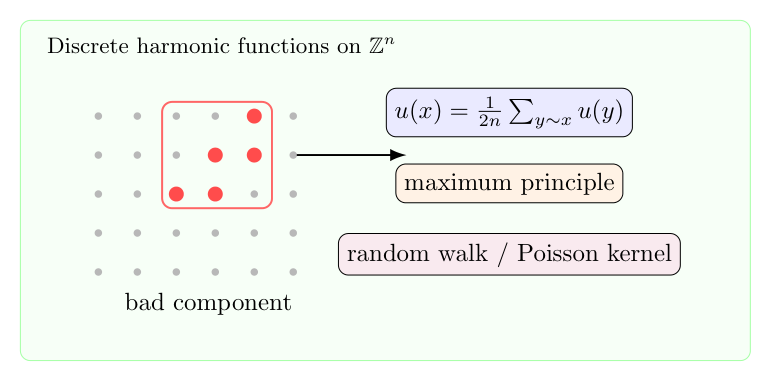
离散调和函数：格点 Laplacian、坏点集合与 Liouville 型问题 — 离散调和函数的平均值性质可以用随机游走解释，坏点集合的几何受到最大值原理控制。

1. 定义

函数 $u:\mathbb Z^n\to\mathbb R$ 称为离散调和，如果对每个 $x\in\mathbb Z^n$，

$$u(x)=\frac1{2n}\sum_{y\sim x}u(y),$$

其中 $y\sim x$ 表示 $y$ 与 $x$ 相邻。等价地，离散 Laplacian

$$\Delta_d u(x)=\sum_{y\sim x}(u(y)-u(x))$$

满足 $\Delta_d u=0$。

在二维中，这就是

$$u(i,j)=\frac14\bigl(u(i+1,j)+u(i-1,j)+u(i,j+1)+u(i,j-1)\bigr).$$

2. 最大值原理

离散调和函数满足最大值原理：如果 $u$ 在有限连通区域内部调和，那么最大值和最小值出现在边界上。原因很简单：一个点的值是邻点平均，若内部点达到严格最大值，则所有邻点也必须取同样的值，连通性迫使整个区域常数。

这使得坏点集合的形状受到限制。设

$$G=\{x:|u(x)|\le 1\},\qquad B=\mathbb Z^n\setminus G.$$

如果某个坏点连通块完全被好点包围，那么最大值原理会迫使它不能真正坏。因此坏点必须以某种方式连接到边界或无穷远。

3. Poisson kernel 与随机游走

在有限区域 $\Omega\subset\mathbb Z^n$ 上，离散调和函数由边界值决定：

$$u(x)=\sum_{z\in\partial\Omega}P_\Omega(x,z)u(z).$$

这里 $P_\Omega(x,z)$ 是从 $x$ 出发的简单随机游走第一次离开 $\Omega$ 时落在 $z$ 的概率。这就是离散 Poisson kernel。

这个表示把分析问题转成概率问题：若边界上大值点所占比例很小，那么内部点看到大值的概率也会受到控制。

4. Liouville 型命题

经典 Liouville theorem 说，有界的整调和函数必须是常数。离散版本也有类似结论。更细的问题是：如果 $u$ 不假设处处有界，但在每个大球里都有固定比例的点满足 $|u|\le 1$，是否仍能推出 $u$ 是常数？

这类命题的证明通常要比较两个方向。第一，离散调和性和 Poisson 表示迫使内部值由边界平均控制。第二，若存在越来越大的坏点连通块，那么等周不等式或随机游走逃逸概率会给出大值传播。二者冲突时，就只能得到常数解。

5. 为什么维数和尺度重要

在 $\mathbb Z^n$ 中，每个半径球只有有限个格点，边界体积和内部体积之间有明确关系。坏点集合若想在所有尺度上保持稀疏，就很难同时支撑一个非平凡调和函数的增长。

这和连续情形的差别在于，离散空间把局部传播路径变成了组合对象。一个值要从边界影响内部，必须沿随机游走路径进入；而路径数量、逃逸概率和等周结构都会参与估计。

6. 证明图像

可以把证明想成两条 lemma 的冲突。一个 lemma 来自 Poisson kernel：内部值是边界值的随机平均，因此不能随意增长。另一个 lemma 来自坏点集合的几何：如果坏点在每个尺度都存在足够结构，它的质量会以某种速率传播。若假设“好点比例”在所有尺度上都足够大，这两种趋势最终矛盾。

这个问题的有趣之处在于，它把调和分析、随机游走和离散等周不等式绑在一起。离散调和函数不是连续理论的机械翻译，而是一种真正带有格点几何味道的分析对象。

分类： Discrete harmonic function

离散调和函数：格点 Laplacian、坏点集合与 Liouville 型问题