分类: Ergodic theory

  • Van der Corput trick:从差分到均匀分布

    旧博客原文

    原题:Van der curpurt trick

    There is the statement of Van der carport theorem:

    Given a sequences \{x_n\}_{n=1}^{\infty} in S_1, if \forall k\in N^*, \{x_{n+k}-x_n\} is uniformly distributed, then \{x_n\}_{n=1}^{\infty} is uniformly distributed.

    I do not know how to establish this theorem with no extra condition, but this result is true at least for polynomial flow.

    |\sum_{n=1}^Ne^{2\pi imQ(n)}|= \sqrt{(\sum_{n=1}^Ne^{2\pi imQ(n)})(\overline{\sum_{n=1}^Ne^{2\pi imQ(n)}})}

    = \sqrt{\sum_{h_1=1}^N\sum_{n=1}^{N-h_1}e^{2\pi imQ(n+h_1)-Q(n)}}=\sqrt{\sum_{h_1=1}^N\sum_{n=1}^{N-h_1}e^{2\pi im \partial^1_{h_1}Q(n)}} \leq \sqrt{\sum_{h_1=1}^N|\sum_{n=1}^{N-h_1}e^{2\pi \partial^1_{h_1}Q(n)}|}

    = \sqrt{\sum_{h_1=1}^N\sqrt{ (\sum_{n=1}^{N-h_1}e^{2\pi \partial^1_{h_1}Q(n)} )(\overline{\sum_{n=1}^{N-h}e^{2\pi \partial^1_{h_1}Q(n)})}}}\leq\sqrt{\sum_{h_1=1}^N\sqrt{ \sum_{h_2=1}^N|\sum_{n=1}^{N-h_1}e^{2\pi\partial^1_{h_2} \partial^1_hQ(n)} |}}

    \leq ....\leq

    \sqrt{\sum_{h_1=1}^N\sqrt{ \sum_{h_2=1}^N \sqrt{....\sqrt{\sum_{h_{k-1}=1}^{N-h_{k-2}}|\sum_{n=1}^{N-h_{k-1}}e^{2\pi\partial_{h_1h_2...h_{k-1}Q(n)}}|}}}} =o(1)


    This type of trick could also establish the following result, which could be understand as a discretization of the Vinegradov lemma.

    Uniformly distribution result of F_p:
    Given Q(n)=a_kn^k+...+a_1n+a_0, \{Q(0),Q(1),...,Q(p-1)\} coverages
     to a uniformly distribution in \{0,1,...,p-1\}
     as p \to \infty.

    This trick could also help to establish estimate of correlation of low complexity sequences and multiplicative function, such as result:

    S(x)=\sum_{n\le x}\left(\frac{n}{p}\right)\mu(n)=o(n)

    Maybe with the help of B-Z-S theorem.

    The standard estimate of Mobius function is:

    \sum_{n\leq X:n\equiv a~(mod~q)} \mu^2(n)=\frac{6}{\pi^2} \prod_{p|q} \left(1-\frac{1}{p^2} \right)\frac{X}{q}+E(X,q,a)

    The error term O_{\varepsilon}\left(\sqrt{X/q} +q^{\frac{1}{2}+\varepsilon}\right) is true for q\leq X^{\frac{2}{3}-\varepsilon}.


    补充说明

    以下是新整理的中文说明;上方旧博客原文保持不变。

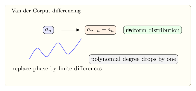
    Van der Corput trick 的核心是:不要直接估计一个振荡平均,而是估计它与平移后的相关。若所有非零差分序列都足够均匀,那么原序列本身也应当均匀。
    Van der Corput trick:从差分到均匀分布
    Van der Corput trick 用差分相关替代原始平均,在多项式相位问题中会降低次数。

    1. 均匀分布版本

    设 $(a_n)$ 是 $\mathbb T^d$ 中的序列。一个典型命题是:若对每个 $h\ne0$,差分序列

    $$a_{n+h}-a_n$$

    都在 $\mathbb T^d$ 中均匀分布,那么 $a_n$ 也均匀分布。证明通常通过 Weyl criterion,把问题化成指数和估计。

    2. 指数和不等式

    对复数序列 $u_n$,Van der Corput 不等式给出

    $$\left|\frac1N\sum_{n\le N}u_n\right|^2
    \lesssim \frac1H+\frac1H\sum_{1\le h\le H}\left|\frac1N\sum_{n\le N-h}u_{n+h}\overline{u_n}\right|.$$

    右侧出现的就是相关项。若相关项都小,则原平均小。

    3. 多项式相位

    当 $u_n=e(P(n))$ 且 $P$ 是次数 $k$ 的多项式时,差分 $P(n+h)-P(n)$ 的次数降为 $k-1$。因此可以用归纳证明 Weyl 型均匀分布结论。

    4. 与乘法函数相关

    在 Mobius 或 Liouville 与低复杂度序列的相关估计中,Van der Corput trick 常用于把一个序列的复杂度下降一层,再配合 Bourgain-Sarnak-Ziegler criterion。它的角色不是给出最终消去,而是把问题改写成更适合结构分析的形式。
  • From periodic to quasi-periodic:周期轨道、无理旋转与逼近

    旧博客原文

    原题:From periodic to quasi periodic

    旧站归档中的这篇正文原本为空。


    补充说明

    以下是新整理的中文说明;上方旧博客原文保持不变。

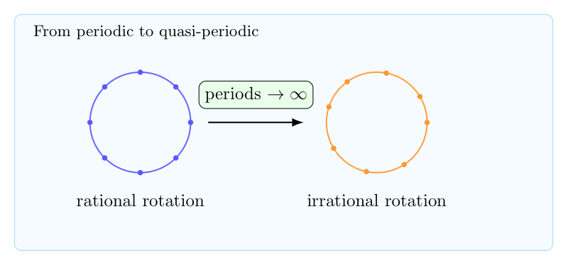
    从 periodic 到 quasi-periodic,最简单的模型是圆周旋转

    $$R_\alpha:x\mapsto x+\alpha\pmod 1.$$

    当 $\alpha=p/q$ 为有理数时,每条轨道都是周期的;当 $\alpha$ 为无理数时,轨道不闭合,而是在圆周上稠密。这两种现象之间由有理逼近连接。

    From periodic to quasi-periodic:周期轨道、无理旋转与逼近
    周期旋转与拟周期旋转之间由有理逼近连接,时间尺度决定了两者看起来有多接近。

    1. 周期轨道

    若 $\alpha=p/q$ 且 $(p,q)=1$,则

    $$R_\alpha^q x=x.$$

    因此动力系统分解成长度为 $q$ 的有限轨道。许多谱量、平均量和相关函数都可以化成有限和。

    2. 拟周期轨道

    若 $\alpha$ 无理,则 $n\alpha$ 模 $1$ 稠密。更强地,Weyl criterion 给出均匀分布:

    $$\frac1N\sum_{n\le N}e^{2\pi i k n\alpha}\to0,\qquad k\ne0.$$

    这说明拟周期不是“没有规律”,而是有一种全局平均意义下的均匀规律。

    3. 有理逼近的两面性

    连分数给出 $\alpha$ 的最佳有理逼近 $p_j/q_j$。在时间尺度 $q_j$ 以下,无理旋转很像周期 $q_j$ 的旋转;但超过这个尺度后,误差积累会显露真正的拟周期行为。

    4. 推广到高维环面

    在 $\mathbb T^d$ 上,平移 $x\mapsto x+\omega$ 的轨道性质由整数关系 $k\cdot\omega$ 控制。没有非平凡整数关系时,轨道稠密;若还满足 Diophantine 条件,则许多小除数估计也会变得可控。

  • 用互不相交闭区间覆盖半开区间:Ostrowski 表示与有效均匀分布

    旧博客原文

    原题:Covering a non-closed interval by disjoint closed intervals

    this note will talk about the Ostrowski representation and approximation by continue fraction.

    As well-known,by the Weyl criterion,\{n\alpha\} is uniformly distribution in [0,1] iff \alpha\in R-Q.

    i.e. we have:\forall 0\leq a\leq b\leq 1,we have:

    \lim_{N\to \infty}|\{1\leq n\leq N|\{n\alpha\}\in [a,b]\}|=(b-a)N+o(N).

    but this will not give the effective version.i.e. we do not the the more information about the decay of o(N).

    we will give a approach of effective version of \alpha with smooth condition by give another proof of the uniformly distribution (in fact to to decomposition the interval [a,b] in to a finite sums of special intervals).and get the result:

    D_N=\int_{M}D_N(\theta)d\mu=\int_Msup_{0<a<b<1}|\sum_{n=1}^{N}\chi_{(a,b)}(\{\theta n \})-N(b-a)|d\mu\sim O(log N)

    if the term in the continuous fraction of \alpha have a up bound.this is so called \alpha is smooth.


    补充说明

    以下是新整理的中文说明;上方旧博客原文保持不变。

    讨论无理旋转 $x\mapsto x+\alpha$ 的均匀分布时,Weyl criterion 告诉我们

    $$\frac1N\sum_{n\le N}e(k n\alpha)\to0,\qquad k\ne0.$$

    但这个判别法本身并不给出非常几何的有效误差。若想知道轨道落入某个区间 $I$ 的次数和 $N|I|$ 相差多少,就需要把区间和时间长度一起分解得更细。

    用互不相交闭区间覆盖半开区间:Ostrowski 表示与有效均匀分布
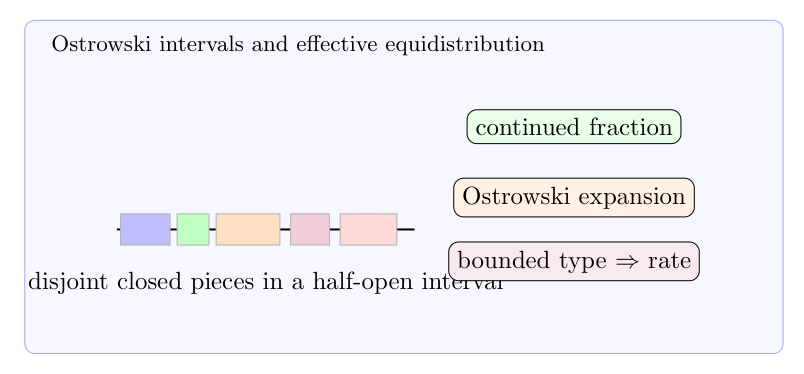
    Ostrowski 表示把轨道长度分解成连分数分母尺度,半开区间也可以拆成有限个互不相交的闭区间来控制端点误差。

    1. 半开区间为什么麻烦

    区间若不是闭的,端点会造成计数上的小麻烦;但在动力系统里,端点通常只贡献有限误差。因此可以把半开区间分解成有限个互不相交的闭区间,再把端点误差单独处理。

    2. 连分数与最佳逼近

    设 $\alpha=[a_0;a_1,a_2,\ldots]$,其收敛分母为 $q_j$。最佳逼近性质说明,长度约为 $\|q_j\alpha\|$ 的小区间正好对应旋转轨道的自然尺度。

    Ostrowski 表示把整数 $N$ 写成

    $$N=\sum_j b_j q_j,$$

    其中系数 $b_j$ 由连分数项控制。于是前 $N$ 次轨道可以分成若干个以 $q_j$ 为长度的块。

    3. 有效均匀分布

    若 $\alpha$ 的连分数项有一致上界,也就是 bounded type,那么每个尺度的坏误差都不会积累得太快。这样可以得到 Denjoy-Koksma 型估计:

    $$\left|\sum_{n

    这就是原来想要的“smooth”或有效版本:不仅知道趋于均匀,还知道偏差怎样增长。

  • Interval map:周期三、Markov 分割与拓扑熵

    旧博客原文

    原题:Interval map

    1.period 3 induce chaos

    theorem:if a interval map T:I\to I have a period 3 point x,then \forall n\in N^*,there is a period n point for T.

    proof:

    n=1 case. trivial

    n>1,n\neq 3 case:

    the key point is to consider the structure of monotone interval contain previous one with fix length.

    this will easy to lead a proof.


    2.a work of J.Milnor and W.Thurston.

    N(T^n) defined as the number of monotone interval of the map T^n.

    theorem:h(T)=lim_{n\to infty}\frac{1}{n}log N(T^n).


    3.monotone Markov map

    this structure have two property:

    1.piesewise monotone and $C^1$,the derive has control!


    there is a relative dynamic system with this map.is a shift map with a relative n\times n matrix A.

    this two dynamic system have a lot of relation,the key one is:

    the topological entropy of monotone Markov map is just the unique maximum eigenvalue of A.

    and some byproduct…


    补充说明

    以下是新整理的中文说明;上方旧博客原文保持不变。

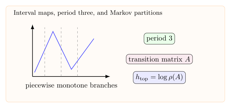
    区间映射是一维动力系统中最能体现“简单空间产生复杂轨道”的模型。一个连续映射 $f:I\to I$ 若有周期三点,就已经含有所有周期的影子,这就是 Li-Yorke 定理背后的核心图像。

    Interval map:周期三、Markov 分割与拓扑熵
    区间映射的复杂性可以通过分段单调结构和 Markov transition matrix 转化为组合增长。

    1. 周期三为什么特别

    设存在 $x$ 使得 $x,f(x),f^2(x)$ 互不相同且 $f^3(x)=x$。三个点在区间上的顺序会迫使某些子区间被映到包含另一些子区间的位置。利用介值定理,可以构造嵌套区间,从而得到任意周期点。

    2. 分段单调与 lap number

    Milnor-Thurston 的一个基本量是 $f^n$ 的单调区间个数,常记作 $\ell(f^n)$。拓扑熵可以由增长率给出:

    $$h_{\rm top}(f)=\lim_{n\to\infty}\frac1n\log \ell(f^n).$$

    这把轨道复杂度转化成组合增长。

    3. Markov 映射

    若区间被分成有限个小区间,且每个小区间在 $f$ 下覆盖若干小区间,就得到一个 transition matrix $A$。对应的符号动力系统是一个 subshift of finite type。

    4. 熵与最大特征值

    在 Markov 情形下,长度为 $n$ 的允许轨道数由 $A^n$ 控制,因此

    $$h_{\rm top}(f)=\log \rho(A),$$

    其中 $\rho(A)$ 是矩阵最大特征值。这样一维动力系统的混沌程度就被线性代数读出来了。