旧博客原文
原题:k-hessian equation and k-curvature equation
here is the problem, how to understand k-hessian equation and k-curvature equation.
k-hessian equation
k-hessian equation is:

where u is admissible, i.e. 

The most important result is the following three:
1.sovable (*) with direchlet boundary condition.
This is mainly the contribution of Caffaralli in 90’s. According flexible function and maximum principle we can establish the 

2.Hessian measure.
This is mainly the work of X.J.Wang and Trudinger. they proved:
in the meaning of viscosity solution, if 


when 

if 

this is merely depend on a priori estimate on
3.pointwise estimate corresponding wolff potential.
the Wolff potential is:

We can easily use rescaling to understand the reasonable of this potential, and use this potential Lubutin establish the following pointwise estimate:


the RHS could look as a corollary of classical A-B-P estimate. the LHS need combine several observation. mean-value property and some else.
This result could use to establish some result on singularity point can be removable.
k-curvature equation
1.sovable (*) with direchlet boundary condition.
This is also established by cafferalli.
2.curvature measure.
This is established very recently. mean curvature equation in 2014, by perron lift and modified, general case in 2016 by more complex calculate and method.
3.pointwise estimate corresponding wolff potential.
This still do not established, and is the main thing I focus on. Due to we can look as k-curvature as a “projection” of k-hessian equation, Calderon-Zegmund decomposition and the estimate of k-hessian equation maybe useful.
My ideas
look is as “average” of “loop space”, “surface space”.
1.Grassmannian bundle
n algebraic geometry, the Grassmann d-plane bundle of a vector bundle E on an algebraic scheme X is a scheme over X:
such that the fiber


Like the usual Grassmannian, the Grassmann bundle comes with natural vector bundles on it; namely, there are universal or tautological subbundle S and universal quotient bundle Q that fit into

Specifically, if V is in the fiber p−1(x), then the fiber of S over V is V itself; thus, S has rank 



which is nothing but a family of Plücker embeddings.
The relative tangent bundle 

which is morally given by the second fundamental form. In particular, when d = 1, the early exact sequence tensored with the dual of S = O(-1) gives:

which is the relative version of the Euler sequence.

2.Explain of the fully nonlinear elliptic equation
Now, we could consider the determination 

Now we need to understand 


where 
But the difficult to make the argument rigorous is that $u_i$ is scale and $e_i$ is vector.
补充说明
以下是新整理的中文说明;上方旧博客原文保持不变。
$k$-Hessian 方程是完全非线性椭圆方程中的基本模型。它把 Hessian 矩阵特征值的第 $k$ 个基本对称函数作为主算子;椭圆性不再自动成立,而是依赖 admissible cone。
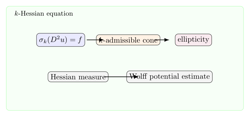
1. 方程与 admissibility
设 $\lambda(D^2u)$ 是 Hessian 的特征值,定义
$$S_k(D^2u)=\sigma_k(\lambda(D^2u)).$$
$k$-Hessian 方程写作
$$S_k(D^2u)=f.$$
为了让方程椭圆,需要要求
$$\lambda(D^2u)\in \Gamma_k=\{\sigma_1>0,\ldots,\sigma_k>0\}.$$
这样的 $u$ 称为 $k$-admissible。这个条件是非线性椭圆理论的入口。
2. Dirichlet 问题
Dirichlet 问题要求
$$S_k(D^2u)=f\quad\text{in }\Omega,\qquad u|_{\partial\Omega}=\varphi.$$
经典策略是建立 $C^0$、梯度和二阶先验估计,再用连续性方法。边界估计通常最细,需要利用 domain 的几何条件、barrier function 和 rescaling。
3. Hessian measure
对非光滑 admissible 函数,也可以定义 Hessian measure。若 $u_j\to u$,并且 $u_j$ 是光滑 admissible,那么在合适条件下
$$S_k(D^2u_j)\,dx \rightharpoonup \mu_k[u].$$
这把方程扩展到 viscosity/pluripotential 风格的弱解框架。它类似 Monge-Ampere measure,但 $k$-Hessian 的 cone 结构更复杂。
4. Wolff potential
点态估计中会出现 Wolff potential:
$$W_{\alpha,p}^\mu(x)=\int_0^\infty\left(\frac{\mu(B(x,r))}{r^{n-\alpha p}}\right)^{1/(p-1)}\frac{dr}{r}.$$
它描述右端测度在不同尺度上的集中。对 $k$-Hessian 方程,解的上下界可以用相应的 Wolff potential 控制。这个形式可以从 scaling 看出:非线性阶数决定了势函数的指数。
5. 与几何曲率方程的联系
$k$-curvature 方程通常把 hypersurface 的第 $k$ 个曲率函数固定下来。解析上它和 Hessian 方程共享 symmetric polynomial、admissible cone 和 fully nonlinear ellipticity。几何问题中的正则性,往往依赖同一套先验估计和弱测度理论。