旧博客原文
原题:Two stupid question
The story of the infinite dimensional space of $\Delta$ is following, we eliminate ourself with compact smooth non-boundary manifold $M$ with metric $g$, then we have Betrami-Laplace operator $\Delta_g$. We could instead $\Delta_g$ by hodge laplace $dd^*+d^*d$, but let we consider $\Delta_g$ the eigenvalue problem:
$$\Delta_g u=\lambda u$$
A classical way to investigate the eigenvalue problem is according to consider variational principle and max-min principle. We equip the path integral on the function space $C^{\infty}(M)$:
$$E(f)=\frac{\int_M |\nabla u|^2}{\int_M |u|^2 }$$
Then it have a sequences of eigenvalue, negative of course: $$0<-\lambda_1<-\lambda_2<…<\lambda_k<…$$
Then things become interesting, the morse theory of infinite space involve, called the infinite space as $X$, so at least, shrink the far place of $X$ as a point, in physics, this mean, cut off at fix scale. And we can take the scale to infinite small, we use the cutoff one to approximation the real one. What I can do is the following, I can proof the eigenvalue function is uniformly distributed in $L^2(M_g)$ (after rescaling of course) and the classical weyl law(although can not give a good error term estimate), but thing become more complicated when I try to consider the infinite space $X_{M_g}$’s topology, at finite scale at least, i.e. $X_{M_g}^{h}$ which is the cut off at scale $h$. Among the other thing, I believe the following issue is true, but without ability to proof it:
>**Problem**
for every manifold $M$ and metric $g$ on $M$, the topology of infinite space $X_{M_g}$ is the same, beside this, the inverse could be true, i.e. If $X_{M_1},X_{M_2}$ is not homomorphism for some scale $h$ then $M_1,M_2$ is not homomorphism.
By intuition, I think it is depend by the underling manifold’s topology. But I do not have a rigorous proof, I definitely have a non-rigorous one, if ignore the coverage…
As I find this problem when I try to give a proof of weyl law, I do not check the reference, may be this problem is a classical one? As always, I will appreciate to any interesting comments and answers, thanks a lots!A
2.
We begin with our favorite situation, the Dirchlet problem on bounded simple-connected domain $\Omega$ in $\mathbb R^n$. Let $\lambda_1$ be the first eigenvalue of $$\Delta u=\lambda u \ in\ \Omega$$
$$u=0\ \ on\ \partial\Omega$$
Rescaling $u$ such that $\sup_{\Omega} u=1$, I think the following property of the first eigenvalue is true.
>**Problem**
We have, the Minkowski functional of $\Omega$, called $M_{\Omega}$ and the Minkowski functional with the ball $B$ such that $vol(B)=vol(\Omega)$, then along the level set of $u$, i.e. the fiber: $$\Omega=\cup_{t\in [0,1]}l_t, l_t:=\{t|x\in \Omega, u(x)=t\}$$
We pretend for the isolate point $l_1$ to be a ball with radius 0, so equipped it with the uniformly density at every direction in $S^1$, i.e. the mass distribution given by $M_B$ and the total mass coincide with the total mass induce by $M_{\Omega}$ in $l_0$, i.e.
$$\int_{e\in S_1}M_{\Omega}(e)d\mu=\int_{e\in S_1}M_{B}(e)d\mu$$
The measure $d\mu$ equipped on $S^1$ is the natural Haar measure. And the cost function is given by $c(x,y)=\|x-y\|^2$. Then, among this setting,
I wish the following property to be true:
Along the direction $1\to 0$, the transport of density $\partial_{t_0} M_{\cup_{t=t_0}^1l_t}$ given the unique optimal transport of the natural measure induce by $M(\Omega)$ and $M(B)$.
**Remark 1** As point out by SebastianGoette, the multiplicity of the first eigenvalue must be one, thanks to the eigenfunction never change the symbol, so we are in the best case.
**Remark 2**:I am not very sure this property could always true, there may be a center example when $\Omega$ is not convex, but I tend to believe it is true at least when $\Omega$ is convex.
**Remark 3**: As point out by Dirk, when you try to consider the optimal transport problem, you always need to point out the cost function $c(x,y)$ defined on $\Omega \times \Omega$, for there, I think the naive choice is $c(x,y)=\|x-y\|^2$
The thing I can proof is the following, the level set of $u$ should be convex by brunn-minkowski inequality, and some type of monotonically property, i.e. more and more like a ball when the level set is more and more shirking smaller form $\partial \Omega$ to the point $f$ arrive maximum.
I will appreciate for any relevant comments and answer, thanks!
补充说明
以下是新整理的中文说明;上方旧博客原文保持不变。
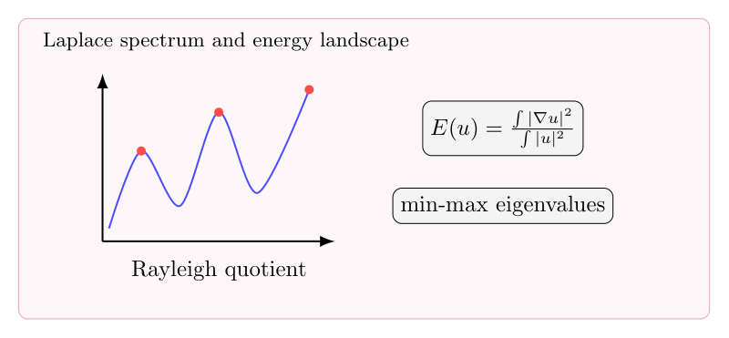
Laplace 特征值问题可以看成无限维函数空间上的变分问题。Rayleigh quotient 的临界点给出 eigenfunctions,min-max principle 给出 eigenvalues。这种图像很像 Morse theory,只是空间变成了无限维。
1. Laplace 特征值问题
在紧无边界 Riemannian manifold 上,考虑
$$-\Delta_g u=\lambda u.$$
谱离散,特征值可以排成
$$0=\lambda_0<\lambda_1\le\lambda_2\le\cdots\to\infty.$$
2. Rayleigh quotient
定义
$$E(u)=\frac{\int_M|\nabla u|^2\,dV_g}{\int_M|u|^2\,dV_g}.$$
在 $L^2$ 单位球上,$E$ 的临界点正是 Laplace eigenfunctions。第一非零特征值是与常数正交的函数中 $E$ 的最小值。
3. Min-max principle
第 $k$ 个特征值可由
$$\lambda_k=\inf_{\dim V=k+1}\sup_{u\in V\setminus\{0\}}E(u)$$
给出。这个公式把谱问题转成函数空间中的拓扑/变分问题。
4. 无限维 Morse 图像
在有限维 Morse theory 中,临界点和拓扑变化有关。Laplace 特征函数也可以看成 Rayleigh quotient 的临界点;其 Morse index 与低于该特征值的谱空间维数相关。
5. 与 Weyl law 的关系
Weyl law 告诉我们高能临界点的数量增长率。变分图像解释 eigenfunctions 从哪里来,Weyl law 则解释这些临界点在高频区域有多密。
 is a compact domain;i.e.
 isometry, the spectrum expansion, ut it still not seems to be chargeable the main difficult come from the compacness this just mean a divide of the whole space, and we consider the X-ray tansigation from every point to the whole space, it need to be passion kernel, or we change it to be a pare matrix.
 for
for  for some eigenvalue
  and all units in this world is the translation and rescaling of u. Then thing become interesting, now how to understand the other guy, i.e. the other eigenvalue and eigenfunctions? They must be the u after some translation combine with rescaling and trslation and rotation!!! so there is a dynamic system action on it! and if we only let it to be affine map,i.e. combine only taslation and rotation, then we just get the all eigenfunctions with the same eigenvalue.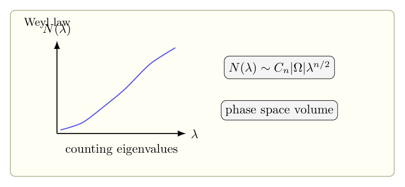
 be a compact
  Riemannian manifold of dimension
  , let
, let  be an
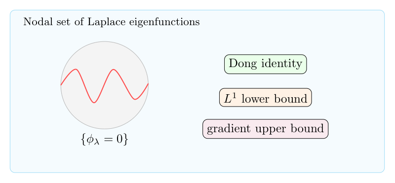
be an  latex N \phi_{\lambda} =\{x:\phi_{\lambda}(x)=0\}$
 denote its
  -dimensional Riemannian hypersurface measure. In this note we prove:
 ,there exists a constant
  so that:
 ,we have,
 ,
,

 ,use divergence theorem:
 in theorem 2,we have:
 ,$||\nabla\phi_{\lambda}||_{\infty}$ ,this two guys are easy to get good estumate….and we will get a lower bound estimate of measure of nodal set:

 norm of