旧博客原文
原题:An approach to Vinogradov estimate
Vinogradov estimate is:

For fix 

Assume 
![([0,1]^n,T)](https://s0.wp.com/latex.php?latex=%28%5B0%2C1%5D%5En%2CT%29&bg=ffffff&fg=5e5e5e&s=0&c=20201002)


First approach
we could easily to get a “uniform distribute on fiber” result without very much tough estimate to attach the theorem. That is just a application by my “rigid trick” that is describe in my early note. But this approach is according to the understanding of the result as a uniformly distribute result on Torus 


Graph
But this approach seems difficult to generate. The difficulty is come from both there is no similar uniformly distribute of the other perimeter use the rigid trick (At least as I know, I try to prove there could be one but I failed) and if in the best case we have the similar uniformly distribute result for other perimeter there is still some thing more need to be established. See this graph for a counterexample that the uniformly distribute for all fiberation could not derive a uniformly distribute for the original space.
Second approach
In this approach we need use the information of continue fractional to get some information (Which is of course critical to get some information about the estimate). But I do not know if it is necessary, maybe this could be a interesting question weather the information come from continue fractional must involve to get such a estimate in the future, but not today.
Any way, there is two different type of continue fractional:
1.
2.
Anyway, these could be understand as a same thing more or less (if fact we can calculate some quantitive with 


Where 


But unfortunately this approximation is too good to be true for 
But for higher degree case, although we could not expect this thing to be true, we still could image a weaker but enough result to be true:

in the Gromov Hausdorff metric sense, and the $T_k^n(x)$ is carefully chose, which have a finite torsion structure(which could be view as a multilinear structure which will play a central role in the estimate). Here is a graph for 
Roughly speaking, in general 
This also have a physics explaining, for which see the graph:
Third approach
For 

补充说明
以下是新整理的中文说明;上方旧博客原文保持不变。
Vinogradov 型估计可以看成带有有效误差的均匀分布定理。若相位含有无理参数,问题往往在两个语言之间切换:动力系统上是环面轨道的均匀分布,解析数论上是指数和的消失。
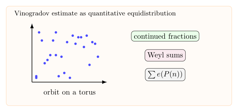
1. 动力系统图像
考虑环面上的序列
$$n\mapsto (n\alpha,n^2\alpha,\ldots)\pmod1.$$
当 $\alpha$ 无理时,这类序列常常均匀分布。Vinogradov 估计要求更强:不仅要知道平均极限,还要给出可用的误差项。
2. 指数和形式
Weyl criterion 把均匀分布转成指数和:
$$\frac1N\sum_{n\le N}e(P(n))\to0.$$
有效估计则要控制
$$\left|\sum_{n\le N}e(P(n))\right|.$$
当 $P$ 的系数包含无理数时,连分数近似会决定哪些尺度上相位最接近有理、哪些尺度上可以得到抵消。
3. Fiber 均匀分布的限制
一种诱人的想法是先证明每个 fiber 上的均匀分布,再合成整个空间的均匀分布。但这并不总是成立:所有纤维方向看起来平均,不代表整体分布没有隐藏相关性。这个失败提示我们必须直接控制整体指数和。
4. 连分数尺度
设 $\alpha$ 的 convergents 是 $p_k/q_k$。在长度接近 $q_k$ 的区间上,$n\alpha$ 的分布有特别好的结构。把 $[1,N]$ 拆成这些标准尺度,可以把任意长度的问题化成一族可估的块。
5. 证明路线
一个合理策略是:先用 Weyl differencing 降低多项式相位阶数;再用连分数控制主要尺度;最后把误差在不同块上求和。动力系统语言提供几何直觉,真正的定量估计则来自指数和技术。