Calderon-Zygmund 分解：奇异积分的实变量入口

旧博客原文

原题：Calderon-Zygmund theory of singular integrals.

1. Calderon-Zygmund decomposition

The Calderon-Zygmund decomposition is a key step in the real variable analysis of singular integrals. The idea behind this decomposition is that it is often useful to split an arbitrary integrable function into its “small” and “large” parts, and then use different technique to analyze each part.

The scheme is roughly as follows. Given a unction and an altitude , we write , where is point wise bounded by a constant multiple . While is large, it does enjoy two redeeming features: it is supported in a set of reasonable small measure, and its mean value is zero on each of the ball that constitute its support. To obtain the decomposition , one might be tempted to “cut” at the height ; however, this is not what works. Instead, one bases the composition on the set where the maximal function of has height .

Theorem 1 (Calderon-Zygmund decomposition)

Suppose we are given a function and a positive number , with . Then there exists a decomposition of , , with , and a sequences of balls , so that,

1. , for a.e. .
2. Each is supported in ,, and .
3. .

 

Before proof this theorem, I explain the geometric intuition why this theorem could be true first. Merely speaking, this is just base on cut off the function into two part, the part with high altitude and the part with low altitude and extension the part with high altitude to make the extension one satisfied the condition 2 and 3.

Proof: In fact this decomposition have a good geometric explain, we just divide the part and extension it carefully to make they behaviour like several balls, to satisfied the special condition on this part.

Remark 1 Remark 1: A Calderon-Zygmund decomposition for function was done in Charlie Fefferman’s thesis; see Section II of ams.org/mathscinet-getitem?mr=257819  One can also find this in Loukas Grafakos’s Classical Fourier Analysis Classical Fourier Analysis page 303 exercise 4.3.8. The question is broken up into parts that should be easy to handle.

Several people have considered with this question. An excellent paper that comes to mind is Anthony Carbery’s Variants of the Calderon–Zygmund theory for -spaces which appeared in Revista Matematica Iberoamericana, Volume 2, Number 4 in 1986. There are also several useful references that appear in Carbery’s paper.

Remark 2 We could also consider a variant of Calderon-Zygmund decomposition, such as equipped with a nontrivial weight function or find some different way to decomposition for some special purpose.

Remark 3 Consider suitable decomposition of the physics space or even both the physics space and fractional space try to gain some reasonable estimate is a fundamental philosophy in harmonic analysis, beside the Calderon-Zegmund decomposition,

Whitney decomposition. Which is important trick in the proof of fefferman-stein restriction theorem and differential topology.

Wave packet decomposition. The wave packet decomposition. This decomposition underlies the proof of Carleson’s theorem (this is more explicit in Fefferman’s proof than Carelson’s original proof), Lacey and Thiele’s proof of the boundedness of the bilinear Hilbert transform, as well as a host of follow-up work in multilinear harmonic analysis. The idea of the wave packet decomposition is to decompose a function/operator in terms of an overdetermined basis. This allows one to preserve symmetries (such as modulation symmetries) that aren’t preserved by a classical Calderon-Zygmund decomposition (which endows the frequency with a distinguished role). One might consider using a wave packet decomposition if is working with an operator that has a modulation symmetry. This is discussed in more detailed in Tao’s blog post on the trilinear Hilbert transform.

Polynomial decomposition. The application of polynomial decomposition to harmonic analysis is more recent, and its full potential still seems unclear. Applications include Dvir’s proof of the finite field Kakeya conjecture, Guth’s proof of the endpoint multilinear Kakeya conjecture (and, indirectly, the Bourgain-Guth restriction theorems), Katz and Guth’s proof of the joints problem and Erdos distance problem, among many other results. Generally, the idea behind the polynomial decomposition is to partition a subset of a vector space over a field into a finite number of cells each of which contains roughly the same fraction of the original set. One further wishes that no low degree algebraic variety can intersect too many of the cells. In Euclidean space, the polynomial ham sandwich decomposition does exactly this. This allows one to, for instance, control linear (or, more generally, `low algebraic degree’) interactions between points in distinct cells. This has so far proven the most useful in incidence-type problems, but many problems in harmonic analysis, thanks to the translation symmetry of the Fourier transform, are inextricably linked with such incidence-type problems. See (again) Tao’s survey of this topic for a more detailed account.

 

2. Singular integrals

Have the Calderon-Zegmund decomposition in hand, now we proof a conditional one bounded result for singular integrals.

The singular integral one is interested in are operator , expressible in the form

 

Where the kernel is singular near , and so the expression is meaningful only if is treated as a distribution or in some limiting sense. Now the particular regularization of may be appropriate depends much on the context, and a complete treatment of the issues thereby raised take us quite far afield.

Let us limit ourselves to two closely related ways of dealing with the questions concerning the definability of the operator. One is to prove estimates for the (dense) subspace where the operator is initially defined. The other is to regularize the given operators by replacing it with a suitable family, and to prove the uniformly estimates for this family. This idea is similar occurring in spectral geometry when we wish to investigate the spectrum of some operator we try to consider some deformation, so deduce to control the spectrum of a seres of paramatrix, for example, consider the wave kernel or heat kernel rather than the passion kernel itself. Common to both methods is a priori approach: We assume some additional properties of the kernel, but then prove estimates that are independent of these “regularity” properties.

We now carry out the first approach in detail. There will be two kinds of assumptions made about the operator. The first is quantitative: we assume that we are given a bound , so that the operator is defined and bounded on with norm ; that is,

 

Moreover, we assume that there is associated to a measurable function (that plays the role of its kernel), so that for the same constant and some constant ,

 

for all .

The further regularity assumption on the kernel is that for each in that has compact surppot, the integral coverages absolutely for almost all in the complement of the support of , and that equality holds for these .

Theorem 2 (Bounded of singular integral with condition)

Under the condition 1 and 3 made above on , the operator is bounded in norm on , when . More precisely,

For with , where the bound depends only on the constant appearing in 1 and 3 and on , but not on the assumed regularity of , or on .

 

Proof:

Now let us begin to prove the conditional theorem. The key point is to use the potential of has been a bounded operator from . Said, it already assumed such that we have . Now let us look at the singular integral expression:

 

 

The key point is to proof the mapping is a weak-type ; that is,

 

At once we establish 5, then the theorem followed by interpolation. Now we use theorem 1 on get , thanks to the triangle inequality and something similar we have , in fact , , by triangle inequality and , to proof , we only need to proof , but this is easy to proof.

Now we know the bounded of , we divide the difficult of establish the weak 1-1 bound of into the difficult of establish the weak 1-1 bound for and . i.e.

 

For , if this weak 1-1 bound is not true, we have,

 

thanks to the trivial estimate . combine this two estimate we have:

 

The first estimate is true on due to . But compare the left and the right of 8 lead a contradiction, so 7 follows. For , the thing is more complicated and in fact really involve the structure of the convolution type of the singular integral. The key point is controlling near the diagonal of . we warm up with a more refine decomposition , . For a large constant choose later define . We know , but the really difficult thing occur in the how to combine the following 5 condition to lead a contradiction:

1. .
2. property come from the Calderon-Zegmund decomposition, and .
3. Hormander condition 3 ,
4. the reverse of weak 1-1 of , .
5. the structure

The first step is to break into , and reduce the case of several balls to the case of only one ball, this could be done by triangle inequality or more may be we could do it derectly, but any way it is not difficult.

Then the thing become intersting, we focus on , divide . thanks to the hormander condition 3 we have good control on , in fact we can proof a weak 1-1 bound on it,

So we conclude,

The last equality used the condition .

 

---

补充说明

以下是新整理的中文说明；上方旧博客原文保持不变。

Calderon-Zygmund 分解是实变量调和分析里最基本的动作之一。它不是简单地把函数按高度截断，而是用 Hardy-Littlewood maximal function 找到真正危险的区域，再把函数分成一个有界的好部分和一族有 cancellation 的坏部分。

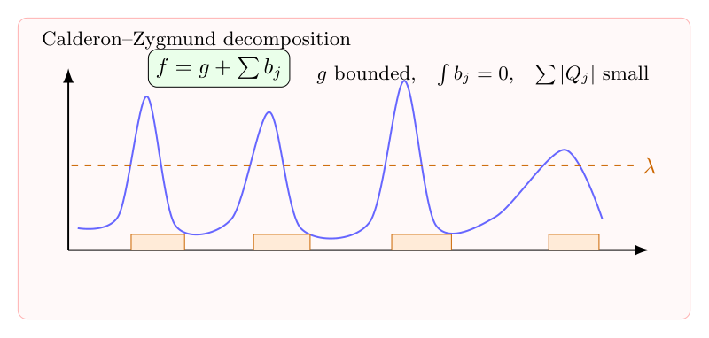
1. 为什么不能直接截断

给定 $f\in L^1(\mathbb R^n)$ 和高度 $\lambda>0$，我们希望写成

$$f=g+\sum_j b_j.$$

其中 $g$ 应该满足 $|g|\lesssim \lambda$，而 $b_j$ 虽然可能很大，但支撑在小集合上，并且有零平均。直接令 $g=f\mathbf 1_{\{|f|\le \lambda\}}$ 并不够，因为奇异积分不是逐点算子，它会感受到坏集合附近的空间结构。

正确做法是看 maximal function 的超水平集：

$$\Omega=\{x:Mf(x)>\lambda\}.$$

然后对 $\Omega$ 做 Whitney decomposition，得到一族彼此控制重叠的 cubes 或 balls。

2. 分解定理

Calderon-Zygmund 分解给出

$$f=g+\sum_j b_j,$$

并且满足：

$$|g(x)|\lesssim \lambda \quad\text{a.e.},$$

$$\operatorname{supp} b_j\subset Q_j,\qquad \int b_j=0,$$

以及

$$\sum_j |Q_j|\lesssim \frac{\|f\|_1}{\lambda},\qquad \sum_j\|b_j\|_1\lesssim \|f\|_1.$$

这里的零平均是关键。奇异积分核在远离 $Q_j$ 的地方可以用光滑性做差分估计，从而把 $b_j$ 的大振幅抵消掉。

3. 用它证明弱 $(1,1)$

设 $T$ 是 Calderon-Zygmund singular integral，并已知 $T$ 在 $L^2$ 上有界。为了证明

$$|\{x:|Tf(x)|>\lambda\}|\lesssim \frac{\|f\|_1}{\lambda},$$

把 $f=g+b$。好部分用 $L^2$ 有界性处理：

$$|\{|Tg|>\lambda/2\}|\lesssim \lambda^{-2}\|g\|_2^2\lesssim \frac{\|f\|_1}{\lambda}.$$

坏部分先丢掉扩大后的坏 cubes，它们总体积可控；在外面利用 $\int b_j=0$ 写

$$Tb_j(x)=\int_{Q_j}\bigl(K(x,y)-K(x,c_j)\bigr)b_j(y)\,dy,$$

再用 kernel 的 Holder 光滑性求和。

4. 更广的分解哲学

Calderon-Zygmund 分解的精神是：在物理空间中识别坏区域，把坏区域局部化，并为每个坏块制造 cancellation。类似思想在 weighted theory、Hardy space、Whitney decomposition、wave packet decomposition 和 polynomial partitioning 中都会出现。

不同分解保留不同对称性。Calderon-Zygmund 分解突出空间局部性；wave packet 分解同时追踪空间和频率；polynomial partitioning 则把几何 incidence 信息放进分析估计里。调和分析很多证明，本质上都是在寻找适合当前算子的分解方式。