分类： Singular integral

旧博客原文

原题：A glimpse to the general theory

1. Introduction

We have talked about a very basic result in singular integral, i.e. if we have an additional condition, i.e. bounded condition, then by interpolation theorem we only need to establish the weak bound then we establish the bound of , .

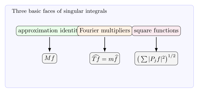
The category of of singular integral is very general, in fact the singular integral we interested in always equipped more special structure. We discuss following 3 types result which world be the central role in this further series note.

1. Approximation of the identity.
2. Singular integral with bounded translation invariant operator.
3. Maximal function, singular integral, and square functions.

The underlying object we consider in both the three case is some special singular integral, in the first case, it looks like a , this, among the other thing, has a close relationship with the maximal operator . This is discussed in 2. For the singular integral with bound, the Fourier transform or its discretization version, Fourier series is natural involved. And there is a “representation theorem” similar to the sprite of Reisz representation theorem, said, roughly speaking, if we consider the bound operator adding the condition of transform invariant, then it is really coinside with the case of our image, the operator must behaviour as a Fourier multiple. This is the contant of famous Mikhlin multiplier theorem, and we discuss some technique difficulty in the process of establishing such a theorem, this is the contact of 3. At last we discuss some deep relationship between three basic underlying intution and objects in harmonica analysis, the Maximal function, singular integral, and square functions. They could all be understanding as tools to understanding the variant complicated emerging in singular integral. But there is definitely some common points. This is the theme of 4. Of course there are some further topic which are also interesting, but I do not want to discuss them here, maybe somewhere else.

2. Approximation of the identity

First topic, we discuss the approximation of the identity, this play a central role in understanding solution of PDE, why, I think a key point is this tools carry a lots of information about the scaling of the space, as it well known, analysis could roughly divide into two parts, “hard analysis” and “soft analysis”, approximation of the identity supply a way to transform a result form “hard analysis” side to “soft analysis” side and reverse. And when it shows its whole power always along with the involving of following Dominate convergence theorem:

Theorem 1 (DCT)

Let be a series of function on measure space , and , and satisfied a controlling condition, i.e. we can find a integrable function , such that , then we know,

 

In fact we have even stronger,

 

This is a standard theorem in real analysis, we give the proof.

Proof: is the point-wise limit of so we know f is measurable and also dominate by , so by triangle inequality we have:

Then the 1 is trivially true, due to a diagonal taking subsequences trick. For more subtle result 2, we need use reverse Fatou theorem to show it is true, roughly speaking we have,

The key point is the first inequality above used the reverse Fatou theorem.

Now we discuss of the main result of the approximation identity. So first we need to define what is a approximation identity. a key ingredient is scaling. i.e. we given a function and consider , and we wish,

 

Whenever , but there need some technique assume to make this intuition to be tight, this lead the following definition.

Definition 2 (Approximation of the identity) Suppose is a fixed function on that is appropriated small at infinity (have good enough decay rate), for example, take,

 

Then we define to be an approximation of the identity.

The key theorem is the following, related the approximation of the indentity with the maximal operator.

Theorem 3

 

For heat kernel, the thing is more subtle.

Theorem 4 [Heat kernel estimate]

 

Remark 1 I know this theorem from Lieb’s book. The power of 4 combine with Plancherel theorem could use to establish the Sobolev inequality, at least for the index .

There are 3 ingredients which cold be useful.

1. the power of Rearrangement inequality involve in the Approximation of indentity operator. we could consider the relationship between and , where is constructed by take the average of on the level set but the foliation of scaling. Intuition seems some monotonic property natural emerge.
2. There is a discretization model, i.e. the toy model on gragh, or we think it as correlation between particles, the key point is the rescaling deformation could be instead by semi group or renormalization property.
3. We consider the more general case, now there is not only one but a group of them, i.e. , this will involve some amenable theory I think.

We give two of the original and most important examples, First, if

where

then is the possion kernel, and,

Gives the solution of the Dirichlet problem for the upper half space,

Namely

 

The second example is the Gaussian kernel,

This time, if , then is a solution of the heat equation,

 

 

3. Singular integral with bounded translation invariant operator

The main result proved in last note about singular integral is a conditional one, guaranteeing the boundedness on for a range , on the assupution that the boundedness on is already known; the most important instance of this occurs when . In keeping with this, we consider bounded linear transformation from to itself that commute with translation. As is well known, such operator are characterized by the existence of a bounded function on (the “multiper”), so that can be realized as,

Where denotes the Fourier transform. Alternatively, at least on test function , can be realized in terms of convolution with a kernel ,

 

Where is the distribution given by . We shall now examine how the theorem with condition on singular integral weill lead to some result of this type of operator. Roughly speaking, it is due to now we know the boundedness on , for technique condition, we need to assume the distribution agree away from the origin with a function that is locally integrable away from the origin with a function that is locally integrable away from the origin; in this case we define the function by . Then 10 implies that,

Whenever is in and has campact support. Tis is the representation of singular integral in the present context. Next, the crucial hormander condition is then equivalent with,

 

for all , where . In this case, the condition 12 have a further understanding, in fact,

Lemma 5

 

or its weaker form, (here is fixed )

imply the hormander condition 12

Proof: Integral by part.

So, now the key point is how do , satisfied such conditions, come about? It turns out that, toughly speaking, such condition on have equivalent versions when sated in terms of the Fourier transform of , namely the multiper . This is transform the difficulties from physics space to fractional space In the future note, we will find a proof of the following Theorem:

Theorem 6 For .

If we assume that,

holds for all , then satisfied 5 for all .

If we assume that satisfied the above inequality for all , where is the smallest integer , then satisfied 12

Remark 2 The multiplier satisfied the second part condition of 6, are called Marcinkiewicz mulltiplier.

 

4. Maximal function, singular integral, and square functions.

 

---

补充说明

以下是新整理的中文说明；上方旧博客原文保持不变。

奇异积分的基本理论不只是 Calderon-Zygmund 分解。真正进入一般理论以后，会反复出现三类对象：approximation of the identity、translation invariant singular integrals，也就是 Fourier multipliers，以及 maximal function 和 square function。

1. 从弱型估计到 $L^p$ 有界性

如果一个奇异积分算子 $T$ 已知在 $L^2$ 上有界，并且满足弱 $(1,1)$ 估计

$$|\{x:|Tf(x)|>\lambda\}|\lesssim \frac{\|f\|_1}{\lambda},$$

那么 Marcinkiewicz interpolation 给出 $1

2. Approximation of the identity

取一族核 $\phi_t(x)=t^{-n}\phi(x/t)$，若 $\int\phi=1$，则

$$\phi_t*f\to f\quad(t\to0).$$

这类算子看起来温和，但它们和 maximal operator 紧密相连。控制

$$\sup_{t>0}|\phi_t*f(x)|$$

本质上就是控制函数在不同尺度上的平均行为。

3. Translation invariant operators

若 $T$ 与平移可交换，那么 Fourier transform 会把它对角化：

$$\widehat{Tf}(\xi)=m(\xi)\widehat f(\xi).$$

Mikhlin multiplier theorem 给出一套可检验条件：若

$$|\partial^\alpha m(\xi)|\lesssim |\xi|^{-|\alpha|}$$

到足够阶数成立，则 $T$ 在 $L^p$ 上有界。

4. Square functions

square function 把函数分解到不同频率或尺度：

$$Sf(x)=\left(\sum_j |P_jf(x)|^2\right)^{1/2}.$$

它不是只估计每一块，而是用正交性追踪所有尺度的总能量。这是 Littlewood-Paley 理论的核心。

5. 一条总线

近似恒等处理尺度极限，multiplier theory 处理平移不变结构，square function 处理多尺度正交性。奇异积分的一般理论，就是在这三种结构之间来回切换。

旧博客原文

原题：Calderon-Zygmund theory of singular integrals.

1. Calderon-Zygmund decomposition

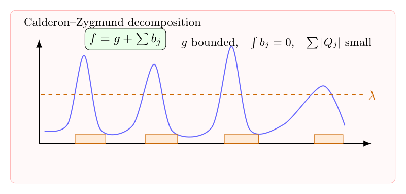
The Calderon-Zygmund decomposition is a key step in the real variable analysis of singular integrals. The idea behind this decomposition is that it is often useful to split an arbitrary integrable function into its “small” and “large” parts, and then use different technique to analyze each part.

The scheme is roughly as follows. Given a unction and an altitude , we write , where is point wise bounded by a constant multiple . While is large, it does enjoy two redeeming features: it is supported in a set of reasonable small measure, and its mean value is zero on each of the ball that constitute its support. To obtain the decomposition , one might be tempted to “cut” at the height ; however, this is not what works. Instead, one bases the composition on the set where the maximal function of has height .

Theorem 1 (Calderon-Zygmund decomposition)

Suppose we are given a function and a positive number , with . Then there exists a decomposition of , , with , and a sequences of balls , so that,

1. , for a.e. .
2. Each is supported in ,, and .
3. .

 

Before proof this theorem, I explain the geometric intuition why this theorem could be true first. Merely speaking, this is just base on cut off the function into two part, the part with high altitude and the part with low altitude and extension the part with high altitude to make the extension one satisfied the condition 2 and 3.

Proof: In fact this decomposition have a good geometric explain, we just divide the part and extension it carefully to make they behaviour like several balls, to satisfied the special condition on this part.

Remark 1 Remark 1: A Calderon-Zygmund decomposition for function was done in Charlie Fefferman’s thesis; see Section II of ams.org/mathscinet-getitem?mr=257819  One can also find this in Loukas Grafakos’s Classical Fourier Analysis Classical Fourier Analysis page 303 exercise 4.3.8. The question is broken up into parts that should be easy to handle.

Several people have considered with this question. An excellent paper that comes to mind is Anthony Carbery’s Variants of the Calderon–Zygmund theory for -spaces which appeared in Revista Matematica Iberoamericana, Volume 2, Number 4 in 1986. There are also several useful references that appear in Carbery’s paper.

Remark 2 We could also consider a variant of Calderon-Zygmund decomposition, such as equipped with a nontrivial weight function or find some different way to decomposition for some special purpose.

Remark 3 Consider suitable decomposition of the physics space or even both the physics space and fractional space try to gain some reasonable estimate is a fundamental philosophy in harmonic analysis, beside the Calderon-Zegmund decomposition,

Whitney decomposition. Which is important trick in the proof of fefferman-stein restriction theorem and differential topology.

Wave packet decomposition. The wave packet decomposition. This decomposition underlies the proof of Carleson’s theorem (this is more explicit in Fefferman’s proof than Carelson’s original proof), Lacey and Thiele’s proof of the boundedness of the bilinear Hilbert transform, as well as a host of follow-up work in multilinear harmonic analysis. The idea of the wave packet decomposition is to decompose a function/operator in terms of an overdetermined basis. This allows one to preserve symmetries (such as modulation symmetries) that aren’t preserved by a classical Calderon-Zygmund decomposition (which endows the frequency with a distinguished role). One might consider using a wave packet decomposition if is working with an operator that has a modulation symmetry. This is discussed in more detailed in Tao’s blog post on the trilinear Hilbert transform.

Polynomial decomposition. The application of polynomial decomposition to harmonic analysis is more recent, and its full potential still seems unclear. Applications include Dvir’s proof of the finite field Kakeya conjecture, Guth’s proof of the endpoint multilinear Kakeya conjecture (and, indirectly, the Bourgain-Guth restriction theorems), Katz and Guth’s proof of the joints problem and Erdos distance problem, among many other results. Generally, the idea behind the polynomial decomposition is to partition a subset of a vector space over a field into a finite number of cells each of which contains roughly the same fraction of the original set. One further wishes that no low degree algebraic variety can intersect too many of the cells. In Euclidean space, the polynomial ham sandwich decomposition does exactly this. This allows one to, for instance, control linear (or, more generally, `low algebraic degree’) interactions between points in distinct cells. This has so far proven the most useful in incidence-type problems, but many problems in harmonic analysis, thanks to the translation symmetry of the Fourier transform, are inextricably linked with such incidence-type problems. See (again) Tao’s survey of this topic for a more detailed account.

 

2. Singular integrals

Have the Calderon-Zegmund decomposition in hand, now we proof a conditional one bounded result for singular integrals.

The singular integral one is interested in are operator , expressible in the form

 

Where the kernel is singular near , and so the expression is meaningful only if is treated as a distribution or in some limiting sense. Now the particular regularization of may be appropriate depends much on the context, and a complete treatment of the issues thereby raised take us quite far afield.

Let us limit ourselves to two closely related ways of dealing with the questions concerning the definability of the operator. One is to prove estimates for the (dense) subspace where the operator is initially defined. The other is to regularize the given operators by replacing it with a suitable family, and to prove the uniformly estimates for this family. This idea is similar occurring in spectral geometry when we wish to investigate the spectrum of some operator we try to consider some deformation, so deduce to control the spectrum of a seres of paramatrix, for example, consider the wave kernel or heat kernel rather than the passion kernel itself. Common to both methods is a priori approach: We assume some additional properties of the kernel, but then prove estimates that are independent of these “regularity” properties.

We now carry out the first approach in detail. There will be two kinds of assumptions made about the operator. The first is quantitative: we assume that we are given a bound , so that the operator is defined and bounded on with norm ; that is,

 

Moreover, we assume that there is associated to a measurable function (that plays the role of its kernel), so that for the same constant and some constant ,

 

for all .

The further regularity assumption on the kernel is that for each in that has compact surppot, the integral coverages absolutely for almost all in the complement of the support of , and that equality holds for these .

Theorem 2 (Bounded of singular integral with condition)

Under the condition 1 and 3 made above on , the operator is bounded in norm on , when . More precisely,

For with , where the bound depends only on the constant appearing in 1 and 3 and on , but not on the assumed regularity of , or on .

 

Proof:

Now let us begin to prove the conditional theorem. The key point is to use the potential of has been a bounded operator from . Said, it already assumed such that we have . Now let us look at the singular integral expression:

 

 

The key point is to proof the mapping is a weak-type ; that is,

 

At once we establish 5, then the theorem followed by interpolation. Now we use theorem 1 on get , thanks to the triangle inequality and something similar we have , in fact , , by triangle inequality and , to proof , we only need to proof , but this is easy to proof.

Now we know the bounded of , we divide the difficult of establish the weak 1-1 bound of into the difficult of establish the weak 1-1 bound for and . i.e.

 

For , if this weak 1-1 bound is not true, we have,

 

thanks to the trivial estimate . combine this two estimate we have:

 

The first estimate is true on due to . But compare the left and the right of 8 lead a contradiction, so 7 follows. For , the thing is more complicated and in fact really involve the structure of the convolution type of the singular integral. The key point is controlling near the diagonal of . we warm up with a more refine decomposition , . For a large constant choose later define . We know , but the really difficult thing occur in the how to combine the following 5 condition to lead a contradiction:

1. .
2. property come from the Calderon-Zegmund decomposition, and .
3. Hormander condition 3 ,
4. the reverse of weak 1-1 of , .
5. the structure

The first step is to break into , and reduce the case of several balls to the case of only one ball, this could be done by triangle inequality or more may be we could do it derectly, but any way it is not difficult.

Then the thing become intersting, we focus on , divide . thanks to the hormander condition 3 we have good control on , in fact we can proof a weak 1-1 bound on it,

So we conclude,

The last equality used the condition .

 

---

补充说明

以下是新整理的中文说明；上方旧博客原文保持不变。

Calderon-Zygmund 分解是实变量调和分析里最基本的动作之一。它不是简单地把函数按高度截断，而是用 Hardy-Littlewood maximal function 找到真正危险的区域，再把函数分成一个有界的好部分和一族有 cancellation 的坏部分。

1. 为什么不能直接截断

给定 $f\in L^1(\mathbb R^n)$ 和高度 $\lambda>0$，我们希望写成

$$f=g+\sum_j b_j.$$

其中 $g$ 应该满足 $|g|\lesssim \lambda$，而 $b_j$ 虽然可能很大，但支撑在小集合上，并且有零平均。直接令 $g=f\mathbf 1_{\{|f|\le \lambda\}}$ 并不够，因为奇异积分不是逐点算子，它会感受到坏集合附近的空间结构。

正确做法是看 maximal function 的超水平集：

$$\Omega=\{x:Mf(x)>\lambda\}.$$

然后对 $\Omega$ 做 Whitney decomposition，得到一族彼此控制重叠的 cubes 或 balls。

2. 分解定理

Calderon-Zygmund 分解给出

$$f=g+\sum_j b_j,$$

并且满足：

$$|g(x)|\lesssim \lambda \quad\text{a.e.},$$

$$\operatorname{supp} b_j\subset Q_j,\qquad \int b_j=0,$$

以及

$$\sum_j |Q_j|\lesssim \frac{\|f\|_1}{\lambda},\qquad \sum_j\|b_j\|_1\lesssim \|f\|_1.$$

这里的零平均是关键。奇异积分核在远离 $Q_j$ 的地方可以用光滑性做差分估计，从而把 $b_j$ 的大振幅抵消掉。

3. 用它证明弱 $(1,1)$

设 $T$ 是 Calderon-Zygmund singular integral，并已知 $T$ 在 $L^2$ 上有界。为了证明

$$|\{x:|Tf(x)|>\lambda\}|\lesssim \frac{\|f\|_1}{\lambda},$$

把 $f=g+b$。好部分用 $L^2$ 有界性处理：

$$|\{|Tg|>\lambda/2\}|\lesssim \lambda^{-2}\|g\|_2^2\lesssim \frac{\|f\|_1}{\lambda}.$$

坏部分先丢掉扩大后的坏 cubes，它们总体积可控；在外面利用 $\int b_j=0$ 写

$$Tb_j(x)=\int_{Q_j}\bigl(K(x,y)-K(x,c_j)\bigr)b_j(y)\,dy,$$

再用 kernel 的 Holder 光滑性求和。

4. 更广的分解哲学

Calderon-Zygmund 分解的精神是：在物理空间中识别坏区域，把坏区域局部化，并为每个坏块制造 cancellation。类似思想在 weighted theory、Hardy space、Whitney decomposition、wave packet decomposition 和 polynomial partitioning 中都会出现。

不同分解保留不同对称性。Calderon-Zygmund 分解突出空间局部性；wave packet 分解同时追踪空间和频率；polynomial partitioning 则把几何 incidence 信息放进分析估计里。调和分析很多证明，本质上都是在寻找适合当前算子的分解方式。