Two extremal problems can share a proof architecture without sharing a proof. Benjamin Bedert’s 2025 breakthrough on large sum-free subsets is additive and Fourier-analytic. A July 2026 manuscript on strongly $2$-primitive sets is multiplicative and hypergraph-theoretic. Their common language is not a transferable sieve, but a four-step design: localize, build a strong object in each local block, prevent leakage between blocks, and add the gains. That comparison points toward the right stability question – and also reveals why the most naive version of stability is false.
Here is the headline before the details. The supplied manuscript claims
$$
F(n)=\pi(n)+\left(\frac{27}{2}+o(1)\right)
\frac{n^{2/3}}{(\log n)^2},
$$
where $F(n)$ is the largest size of a strongly $2$-primitive subset of $[1,n]$. One might expect every near-extremizer to be close to the construction behind this formula: almost all primes, plus products of three primes near $n^{1/3}$ arranged as a nearly saturated linear $3$-uniform hypergraph. That literal statement is false. There is, however, an exact and useful replacement: after contracting harmless private-prime lifts, every near-extremizer has a canonical prime layer and a small exceptional hub carrying the entire second-order excess. If the residual hub is mostly made of squarefree triples, then pair saturation and $n^{1/3}$-scale stability follow. Proving – or refuting – that triple-core hypothesis is the remaining inverse problem.
1. Two problems that look similar only from far away
1.1 The sum-free extraction problem
A set $B\subset\mathbb Z$ is sum-free if it contains no $x,y,z$, not necessarily distinct, with
$$x+y=z.$$
For a finite set $A$ of integers, write
$$
S(A)=\max\{|B|:B\subseteq A,\ B\text{ is sum-free}\},
$$
and, for $N$-element sets of positive integers,
$$
S(N)=\min_{|A|=N}S(A).
$$
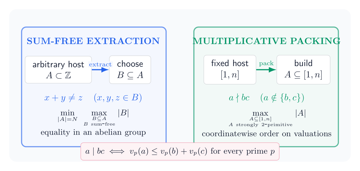
This is an extraction problem. An adversary gives us an arbitrary host set $A$, and we must find a large structured subset inside it. Erdős’s middle-third argument gives $S(A)\ge |A|/3$. Alon and Kleitman improved this to $(N+1)/3$, and Jean Bourgain proved $S(N)\ge (N+2)/3$ in 1997. The long-standing qualitative question was whether the additive improvement can tend to infinity:
$$S(N)\ge \frac N3+\omega(N),\qquad \omega(N)\longrightarrow\infty.$$
Bedert answered yes, proving that an absolute $c\gt0$ exists such that
$$
S(A)\ge \frac{|A|}{3}+c\log\log |A|.
$$
1.2 The strongly $2$-primitive packing problem
A set $A\subseteq[1,n]$ is strongly $2$-primitive when
$$
a\nmid bc
\qquad
(a,b,c\in A,\ a\notin\{b,c\}),
$$
where $b=c$ is allowed. The word strongly matters. Under a more recent convention, a $2$-primitive set only forbids witnesses $b,c$ that are distinct. For example, $\{4,5,6\}$ passes that weaker test but fails the strong one because $4\mid6^2$.
Now define
$$
F(n)=\max\{|A|:A\subseteq[1,n],\ A\text{ is strongly }2\text{-primitive}\}.
$$
This is a packing problem. The host interval is fixed, and we directly construct the largest possible forbidden-divisibility family. The all-primes set gives the leading term $\pi(n)$. In 1938 Erdős proved upper and lower bounds of the form
$$
\pi(n)+c_1\frac{n^{2/3}}{(\log n)^2}
\le F(n)\le
\pi(n)+c_2\frac{n^{2/3}}{(\log n)^2},
$$
and later asked whether the second-order term has an asymptotic constant. This is the modern Erdős Problem #793. The supplied 2026 manuscript proposes that the constant is $27/2$; it is important not to say that Erdős himself conjectured this numerical value.
1.3 Equality versus order
The relation $a\nmid bc$ is not ordinary product-freeness. The set $\{6,10,15\}$, for instance, has no internal equality $xy=z$, yet $6\mid10\cdot15$. Prime valuations expose the real geometry:
$$
a\mid bc
\quad\Longleftrightarrow\quad
v_p(a)\le v_p(b)+v_p(c)
\quad\text{for every prime }p.
$$
Thus the forbidden relation is a coordinatewise domination inequality in the divisor lattice. For squarefree integers, if $E_a=\{p:p\mid a\}$, it becomes
$$E_a\subseteq E_b\cup E_c.$$
So the natural combinatorial object is a $2$-cover-free family, not the solution set of a linear equation. Fourier characters are superb at detecting equations such as $x+y=z$. They do not come with an evident contractive projection that detects the partial order $\nu(a)\le\nu(b)+\nu(c)$. This is the first reason Bedert’s proof cannot simply be copied into the multiplicative setting.
2. The $27/2$ upper bound: every element needs a private factor
Set
$$
y=n^{1/3},\qquad
M=\frac{y}{\log n},\qquad
\Sigma_n=M^2=\frac{n^{2/3}}{(\log n)^2}.
$$
The upper bound begins with a small lemma that contains more information than the inequality it proves.
Think of $E_a=\{u_a,v_a\}$ as a two-element multiset. If $u_a\ne v_a$ and neither coordinate is private to $a$, another chosen pair contains $u_a$ and another contains $v_a$; the corresponding two elements have product divisible by $a$. If $u_a=v_a=x$, failure of privacy would give another pair containing $x$ twice, hence another element equal to $x^2=a$. Therefore every $a$ has a private coordinate, and these coordinates are distinct. That is the injection $A\hookrightarrow\mathcal B$.
The manuscript chooses the multiplicative $2$-basis
$$
\begin{aligned}
\mathcal B_0&=[1,n^{3/5}],\\
\mathcal B_1&=\{p\text{ prime}:n^{3/5}\lt p\le n\},\\
\mathcal B_2&=\{pq:p,q\le y\text{ prime}\},\\
\mathcal B_3&=\{qr:y\lt q\le n^{2/5},\ r\le n/q^2,\ q,r\text{ prime}\}.
\end{aligned}
$$
Every $m\le n$ can be factored into two elements of $\mathcal B=\mathcal B_0\cup\mathcal B_1\cup\mathcal B_2\cup\mathcal B_3$. The case split is elementary but carefully tuned. Small $m$ can be balanced into two factors below $n^{3/5}$, a prime factor above $n^{2/5}$ can be split off, and the remaining difficult case groups two of the three largest prime factors into an element of $\mathcal B_2$ or $\mathcal B_3$.
The main prime layer comes from $\mathcal B_1$. The genuinely second-order counts are
$$
|\mathcal B_2|
=\binom{\pi(y)+1}{2}
=\left(\frac92+o(1)\right)\Sigma_n,
$$
because $\pi(n^{1/3})\sim3n^{1/3}/\log n=3M$, and
$$
|\mathcal B_3|
=\sum_{y\lt q\le n^{2/5}}\pi\!\left(\frac n{q^2}\right)
=(9+o(1))\Sigma_n.
$$
The contribution of $\mathcal B_0$ and all relevant overlaps is $o(\Sigma_n)$. Hence
$$
|\mathcal B|
=\pi(n)+\left(\frac92+9+o(1)\right)\Sigma_n
=\pi(n)+\left(\frac{27}{2}+o(1)\right)\Sigma_n.
$$
The private-factor injection then gives the upper bound. A caution that becomes crucial for stability: $\mathcal B_2$ and $\mathcal B_3$ are labels in an upper-bound certificate. Near-saturation of these labels does not immediately say that the original elements of $A$ are themselves products of two or three primes.
3. The lower bound: turn properly coloured edges into prime triples
The lower bound lives in a linear $3$-uniform hypergraph. Let $\mathcal H$ be a family of triples of distinct primes such that any two triples share at most one prime and every edge product is at most $n$. Define
$$
A_{\mathcal H}
=\{p\le n:p\text{ prime and }p\notin V(\mathcal H)\}
\cup
\left\{\prod_{p\in E}p:E\in\mathcal H\right\}.
$$
Then
$$|A_{\mathcal H}|=\pi(n)-|V(\mathcal H)|+|\mathcal H|.$$
Why is this strongly $2$-primitive? A target triple product has three distinct prime coordinates. Each other hyperedge supplies at most one of them, so two other elements supply at most two. The same argument still works when the two witnesses coincide. Primes outside the vertex set remain singleton elements and cannot divide any other chosen element.
3.1 Logarithmic prime bins
Fix a small mesh $h\gt0$ and divide primes near $y=n^{1/3}$ into bins
$$
P_i=\{p\text{ prime}:ye^{ih}\lt p\le ye^{(i+1)h}\},
\qquad
\Delta_i=e^{(i+1)h}-e^{ih}.
$$
For a cell satisfying
$$i\le j,\qquad i+2j\le-4,$$
put $k=-i-j-3$. Then $i\le j\lt k$, and any $p\in P_i$, $q\in P_j$, $r\in P_k$ obeys $pqr\le n$.
If $i\lt j$, properly edge-colour the complete bipartite graph between $P_i$ and $P_j$, using primes of $P_k$ as colours. When $i=j$, do the same with the complete graph on $P_i$. The lower pair $\{p,q\}$, coloured by $r$, becomes the hyperedge $\{p,q,r\}$.
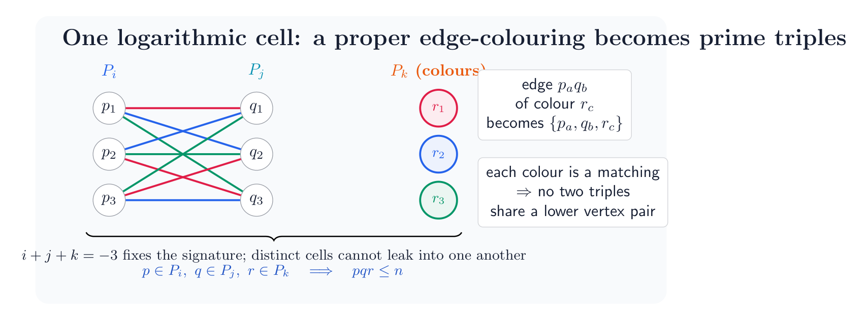
The proper colouring is the local no-interference mechanism. The constant-sum signature is the global one. Together they make the union over all cells a linear hypergraph.
3.2 The cell weight
For any fixed finite collection of bins, the prime number theorem gives
$$|P_i|=(3+o(1))M\Delta_i.$$
Off the diagonal, a cell contributes approximately $9M^2\Delta_i\Delta_j$ edges. A diagonal cell contributes half as many unordered pairs. The exact geometric-series identity is
$$
\sum_{\substack{i\lt j\\i+2j\le-4}}\Delta_i\Delta_j
+\frac12\sum_{i\le-2}\Delta_i^2
=e^{-h}+\frac12e^{-2h}.
$$
Letting $h\to0$, the weight tends to $3/2$, so
$$
|\mathcal H|
=\left(9\cdot\frac32-o(1)\right)\Sigma_n
=\left(\frac{27}{2}-o(1)\right)\Sigma_n.
$$
The number of vertices used is only $o(\Sigma_n)$. Replacing those primes by the triple products therefore yields the matching lower bound.
4. From Erdős’s middle third to Bedert’s $c\log\log N$
We now return to the additive problem. Let $\mathbb T=\mathbb R/\mathbb Z$, and let $\phi=\mathbf1_{(1/3,2/3)}$. The middle third of the circle is sum-free: two points in it cannot add, modulo $1$, to another point in it. Therefore, for every $x\in\mathbb T$,
$$A_x=\{a\in A:ax\pmod1\in(1/3,2/3)\}$$
is sum-free. Averaging $|A_x|$ over $x$ gives $|A|/3$. The problem is to force a positive fluctuation above that mean.
After a harmless normalization, the relevant Fourier series has the form
$$
F_A(x)=\sum_{a\in A}\sum_{m\ge1}
\frac{\chi(m)}m\cos(2\pi max),
$$
where $\chi$ is the non-principal real character modulo $3$. A lower bound for $\|F_A\|_1$ gives a one-sided large value and hence a large sum-free subset.
4.1 Where Bourgain’s sieve loses a logarithm
The historical correction is worth making explicit. The relevant predecessor is Jean Bourgain’s 1997 paper, not “John Bogan, 1993.” Also, the Littlewood $L^1$ conjecture had already been proved in 1981, independently by McGehee-Pigno-Smith and Konyagin. Bourgain’s argument combines Fourier analysis with a Möbius operation that filters harmonic indices.
Schematically, if $R_Q$ denotes the positive $Q$-rough integers, then
$$
\sum_{d\mid\prod_{p\le Q}p}
\frac{\mu(d)\chi(d)}d F_A(dx)
=\sum_{a\in A}\cos(2\pi ax)+\mathcal R_Q(x).
$$
The left side costs
$$
\prod_{p\le Q}\left(1+\frac1p\right)\asymp\log Q
$$
under the triangle inequality. If $Q$ is large enough to make the rough remainder negligible directly, this factor consumes the logarithm delivered by a Littlewood-type lower bound. This explains why merely “using the Littlewood theorem harder” does not produce the desired unbounded gain.
4.2 Bedert’s split: medium primes are sieved, small primes are projected
Bedert chooses
$$Q_1=(\log N)^{1/2},\qquad Q=(\log N)^{20}.$$
He Möbius-sieves only the medium primes $Q_1\le p\le Q$. Their reciprocal sum is $O(1)$, so the norm loss is a constant rather than a logarithm. The small primes $p\le Q_1$ are handled by a different operation.
For every small prime, record the exact valuation $\nu_p(a)$ and the unit residue after removing that prime power. Chinese remaindering packages all this data into a joint fibre $A(r,\nu)$. Fourier projection to a residue class,
$$
\operatorname{Proj}(H;\rho\bmod q)(x)
=\sum_{m\equiv\rho\ (q)}\widehat H(m)e(mx),
$$
is an $L^1$-contraction:
$$
\|\operatorname{Proj}(H;\rho\bmod q)\|_1\le\|H\|_1.
$$
At the main valuation level, the projection removes small-prime harmonic contamination without paying the full Möbius product. After truncation, one sees a large exponential sum plus an $L^2$-small error, to which a robust McGehee-Pigno-Smith test function applies.
At a general valuation level, lower fibres can still leak into the projected channel. Bedert proves an isolation-or-descent alternative: either the desired $L^1$ lower bound is already present, or a large fibre has a strictly lower fibre losing at most a controlled polylogarithmic factor. Iterating and reversing this descent produces a chain
$$
\nu^{(1)}\prec\nu^{(2)}\prec\cdots\prec\nu^{(J)},
\qquad
J\gg\frac{\log N}{\log\log N},
$$
whose fibre sizes grow geometrically.
4.3 The non-Archimedean no-leakage lemma
Associate to these levels the nested moduli
$$
q_i=\prod_{p\le Q_1}p^{\nu_p^{(i)}+1},
\qquad q_1\mid q_2\mid\cdots\mid q_J.
$$
Let $g_i$ be the normalized indicator of the $i$-th residue block and put $Q_i(x)=\exp(-|\widehat g_i(x)|)$. The non-Archimedean MPS test function is assembled from
$$
\Phi_J=
\widehat g_J+\widehat g_{J-1}Q_J+\cdots+
\widehat g_1Q_2\cdots Q_J.
$$
The decisive observation is that $|\widehat g_i|$ is $1/q_i$-periodic, hence $\widehat Q_i$ is supported on $q_i\mathbb Z$. Multiplying an earlier block by a later $Q_k$ shifts its frequencies only by multiples of $q_k$. Since $q_i\mid q_k$, the earlier block cannot escape its residue class modulo $q_i$. Main inner products contribute one controlled unit per block, while geometric fibre growth makes the cross terms summable.
That is Bedert’s genuine no-leakage mechanism. It is more precise than the slogan “use many congruence classes and patch them.”
One further qualification prevents a common misstatement. Bedert obtains a suitable $F_4$-isomorphic model $B$ of the original set and proves the required $L^1$ bound there. The norm $\|F_A\|_1$ is not claimed to be invariant under an $F_4$-isomorphism. What is preserved is the four-term additive information needed for sum-freeness, so $S(A)=S(B)$.
Bedert’s inverse output is also stronger than the numerical lower bound. If $S(A)\le N/3+C$, his results force low additive dimension, a dense $F_4$-model, large additive energy in every substantial subset, and a “99% Structure Theorem” decomposing all but a small exceptional set into large small-doubling pieces. This is a genuine inverse theorem for host sets resisting sum-free extraction, but not an edit-distance classification by one canonical extremizer.
5. The real bridge: localize, build, prevent leakage, sum
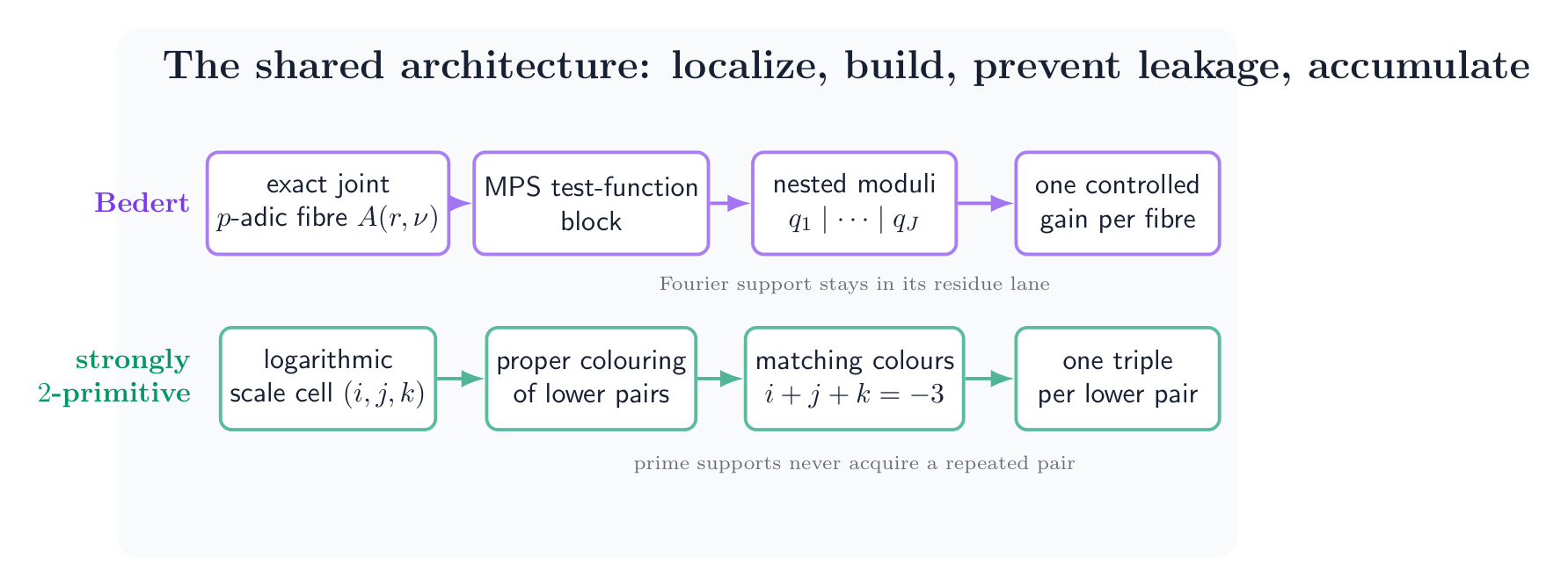
The dictionary is now clean:
| Role | Bedert’s sum-free proof | Strongly $2$-primitive proof |
|---|---|---|
| Underlying relation | Linear equation in an abelian group | Coordinatewise domination of prime valuations |
| Local coordinates | Exact small-prime valuations and unit residues | Logarithmic sizes of prime factors |
| Local block | Joint $p$-adic fibre and MPS block | Scale cell and properly coloured graph |
| No interference | Nested moduli preserve Fourier support | Colour matchings and unique cell signatures preserve linearity |
| Accumulation | One controlled inner product per fibre | One triple per admissible lower pair |
| Inverse output | Additive dimension, energy, small-doubling pieces | Private factors and a cover-free exponent core |
This is a substantial connection, but it is a connection of proof design. Bedert’s Fourier projection has no direct analogue for the divisor partial order. The most plausible transfer is therefore not a line-by-line proof but a research program: find a multiplicative localization, an isolation-or-descent alternative, and a no-leakage invariant that survives repeated prime powers and larger supports.
6. The first stability guess is false
The lower construction suggests a tempting statement: every set with
$$
|A|\ge
\pi(n)+\left(\frac{27}{2}-o(1)\right)\Sigma_n
$$
should differ in only $o(\Sigma_n)$ places from almost all primes plus a near-optimal linear family of triple products. Two examples show why this is too rigid.
6.1 A private-prime lift
Start with a near-optimal linear triple family $\mathcal H_n$ using odd primes below $n/2$. Keep primes above $n/2$, replace every unused prime $p\le n/2$ by $2p$, and retain the triple products. Each $2p$ has the private prime divisor $p$; no other chosen element contains that prime. The triple products are still protected by linearity. The new set remains strongly $2$-primitive and has the same second-order asymptotic size.
But essentially every prime below $n/2$ has been replaced by a composite. The symmetric-difference distance from the all-primes model is
$$
\Theta(\pi(n/2))=\Theta\!\left(\frac n{\log n}\right),
$$
and
$$
\frac{\pi(n/2)}{\Sigma_n}
\asymp n^{1/3}\log n\longrightarrow\infty.
$$
So literal edit-distance stability fails by much more than the scale of the second-order term.
6.2 A nonlinear sunflower at almost no cost
Even if we insist on squarefree triple products, linearity need not hold in the original representation. Add a sunflower
$$\{\{2,3,r\}:r\in R\}$$
for many private petals $r$. Remove the singleton primes $2,3,r$ and add the products $6r$. The net cardinality loss is only $2$, while the support family contains $\asymp n/\log n$ edges sharing the pair $\{2,3\}$. It is $2$-cover-free because every target has its own private petal, but any linear subfamily contains at most one sunflower edge.
The two examples have the same cause: degree-one prime coordinates carry a huge amount of neutral decoration. Stability can only become true after quotienting out this freedom.
7. Near equality in the upper bound is an exact star forest
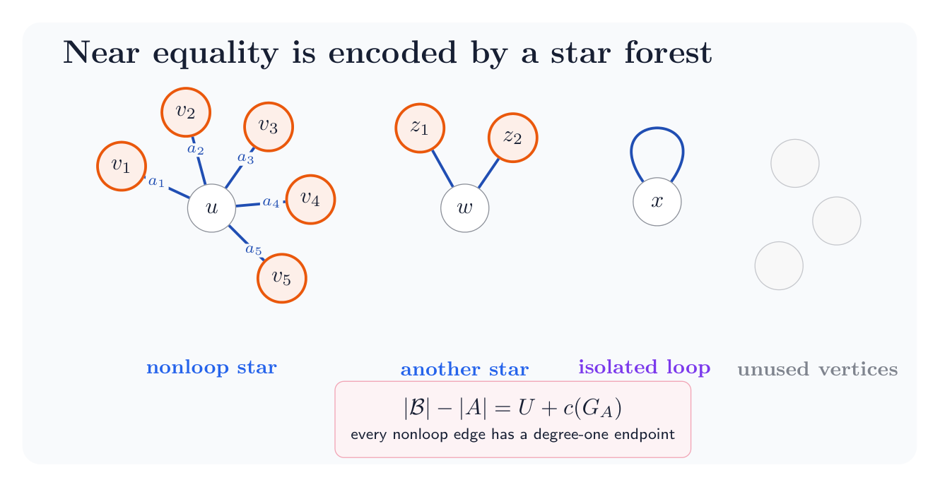
Fix the chosen factorizations $a=u_av_a$ from the multiplicative basis proof. Make a graph $G_A$ with vertex set $\mathcal B$, one edge $\{u_a,v_a\}$ for each $a\in A$, and allow loops.
The proof is the private-factor lemma read without discarding information. If a nonloop edge $\{u,v\}$ had both endpoints in other edges, the corresponding two elements would have product divisible by $uv=a$. If a loop at $u$ met another edge, then $u^2$ would divide the square of the other element.
More quantitatively,
$$
\bigl|\{b\in\mathcal B\setminus\mathcal B_0:
\deg_{G_A}(b)\ne1\}\bigr|
\le |\mathcal B|-|A|.
$$
If
$$
|A|\ge
\pi(n)+\left(\frac{27}{2}-\delta_n\right)\Sigma_n,
$$
then the defect $D_n=|\mathcal B|-|A|$ is at most $(\delta_n+o(1))\Sigma_n$. Hence almost every secondary coordinate in both $\mathcal B_2$ and $\mathcal B_3$ occurs in exactly one chosen factor pair. This is a rigorous stability theorem for the upper-bound certificate. It is not yet a classification of the original integers.
8. Private-prime compression gives the correct normal form
Suppose a prime $p$ divides $a\in A$ and divides no other element of $A$. Replacing $a$ by $p$ preserves the cardinality and strong $2$-primitivity. The new target $p$ cannot divide a product of two other elements because neither contains $p$; for any unchanged target, replacing $a$ by a divisor only decreases the product available to cover it.
For primes $p\gt n^{3/5}$, the basis factorization can be chosen to expose $p$ in every multiple. Thus a degree-one large-prime coordinate is genuinely a globally private prime and can be contracted. Contract all such coordinates simultaneously.
$$\widetilde A=(\mathbb P\cap[1,n]\setminus V)\cup C,\qquad \operatorname{supp}(c)\subseteq V\quad(c\in C).$$
where
$$|V|\le(\delta_n+o(1))\Sigma_n,\qquad |C|-|V|=|A|-\pi(n).$$
In particular, if $\delta_n=o(1)$, then
$$
|V|=o(\Sigma_n),
\qquad
|C|=\left(\frac{27}{2}+o(1)\right)\Sigma_n.
$$
The geometry is now transparent. Before compression, the leading $\pi(n)$ coordinates may be represented by arbitrary private multiples. After compression, almost every prime appears literally. Every residual composite is supported entirely on the small exceptional prime hub $V$, and its excess over the missing primes is exactly the second-order gain.
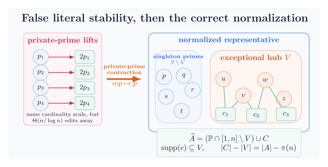
There is one more unconditional consequence. At most $|V|$ members of $C$ have support of size at most two. Indeed, any one- or two-prime residual element must have a valuation coordinate in which it is a strict global maximum; assign the element to such a prime. Two elements cannot receive the same prime. Therefore, in a normalized near-extremizer, all but $o(\Sigma_n)$ residual composites have at least three distinct prime divisors.
This is close to the hoped-for triple picture, but it does not prove that the typical element has exactly three prime factors, that it is squarefree, or that its prime factors lie near $n^{1/3}$.
9. Conditional stability when the residual core is made of triples
Now impose an additional hypothesis:
Let $\mathcal H$ be the support family of those triples. Strong $2$-primitivity says precisely that it is $2$-cover-free:
$$
E\nsubseteq F\cup G
\qquad(E,F,G\in\mathcal H,\ E\notin\{F,G\}),
$$
with $F=G$ allowed.
9.1 Pruning to a linear core
If two triples $E,F$ share a pair and $x$ is the third vertex of $E$, then $x$ has degree one. Otherwise another edge $G$ containing $x$, together with $F$, would cover $E$. Delete such a petal edge whenever a repeated pair occurs. Every deletion removes at least one vertex as well as one edge, so the excess $|\mathcal H|-|V(\mathcal H)|$ does not decrease.
The result is a linear subfamily $\mathcal L$ with
$$
|\mathcal L|-|V(\mathcal L)|
\ge |\mathcal H|-|V(\mathcal H)|,
$$
and only $o(\Sigma_n)$ edges are lost in the normalized near-extremal setting. Notice the nuance: linearity is recovered after pruning private petals; it is not asserted for every cover-free representation.
9.2 Saturating the feasible pair space
Define
$$
\mathcal D_n=
\{(p,q):p\lt q\text{ prime and }pq^2\le n\}.
$$
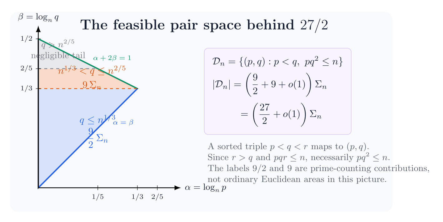
Sort an edge of $\mathcal L$ as $p\lt q\lt r$ and map it to $(p,q)$. Linearity makes this map injective. Since $r\gt q$ and $pqr\le n$, the image lies in $\mathcal D_n$. Direct counting gives
$$
|\mathcal D_n|
=\left(\frac{27}{2}+o(1)\right)\Sigma_n.
$$
The range $q\le n^{1/3}$ contributes $(9/2+o(1))\Sigma_n$; the range $n^{1/3}\lt q\le n^{2/5}$ contributes $(9+o(1))\Sigma_n$; the tail is negligible. Since the linear core already has $(27/2-o(1))\Sigma_n$ edges, its lower-pair map misses only $o(\Sigma_n)$ feasible pairs.
Moreover, for every fixed $\varepsilon\gt0$, all but $o(\Sigma_n)$ edges satisfy
$$
n^{1/3-\varepsilon}
\le p,q,r\le
n^{1/3+\varepsilon}.
$$
This is the desired scale stability. It does not imply uniqueness. Different one-factorizations or different proper edge-colourings can change $\Theta(\Sigma_n)$ triples while preserving the same pair occupancy and extremal count. The stable object is the saturated pair space, not an individual colouring.
10. The remaining inverse problem is weighted and cover-free
After normalization, write every $c\in C$ as an exponent vector
$$
\nu(c)=(v_p(c))_{p\in V}\in\mathbb Z_{\ge0}^{V}.
$$
Strong $2$-primitivity becomes the weighted cover-free condition
$$
\nu(c)\nleq\nu(c_1)+\nu(c_2)
\quad\text{coordinatewise}
$$
whenever $c\notin\{c_1,c_2\}$. We know that
$$
|C|=\left(\frac{27}{2}+o(1)\right)\Sigma_n,
\qquad |V|=o(\Sigma_n),
$$
and that almost every vector has support at least three. What remains unknown is the sharper assertion
$$
\#\{c\in C:c\text{ is not a squarefree product of three primes}\}
=o(\Sigma_n).
$$
This gap may conceal genuine alternative near-extremizers. If a triple $pqr$ has product slack, one can contemplate replacing it by $2pqr$ while deleting the singleton prime $2$. For a linear support family, the underlying three private coordinates still prevent coverage. It is not known whether a positive density of such bounded-hub multiplier layers can coexist globally near the $27/2$ threshold, or whether cross-layer collisions force them to be negligible.
10.1 What a Bedert-style descent would need
The additive proof suggests three design requirements, not three ready-made lemmas.
- A local order projection. One needs to isolate a valuation or support layer while controlling contamination from lower exponent vectors. A divisor-lattice zeta or Möbius transform is a possible language, but no analogue of Bedert’s $L^1$-contractive residue projection is presently available.
- An isolation-or-descent alternative. If the secondary basis slots do not have predominantly prime cofactors, the argument should descend to a structured hub of repeated factors with a quantitative gain or a summable loss.
- A no-leakage invariant. Low codegree and scale signatures work for squarefree triples. A general invariant must survive repeated exponents and supports of size at least four.
The star-forest theorem is already a first inverse statement of this kind: near equality forces almost every basis coordinate to be a leaf attached to a small collection of hubs. The hard step is to turn that certificate-level hub structure into a classification of the original weighted exponent vectors.
11. What is proved, conditional, and open
- Published/preprint additive result: Bedert proves $S(A)\ge |A|/3+c\log\log|A|$, together with inverse information involving additive dimension, dense $F_4$-models, energy and a $99\%$ decomposition into large small-doubling pieces.
- Supplied 2026 manuscript: the claimed $27/2$ asymptotic follows from the multiplicative-basis upper bound and the logarithmic-cell hypergraph construction described above. The status caveat at the beginning remains in force.
- Unconditional stability developed in the accompanying note: literal edit stability is false; the upper-bound factor graph is an exact star forest; private-prime compression gives the normal form $(\mathbb P\setminus V)\cup C$; and almost every residual composite has at least three distinct prime divisors.
- Conditional stability: if almost all residual composites are squarefree triples, pruning gives a near-maximal linear core whose lower pairs saturate $\mathcal D_n$, and almost every prime factor lies at scale $n^{1/3+o(1)}$.
- Open: prove that the normalized residual core is predominantly squarefree of support three, or construct a different near-extremal weighted cover-free core.
The conceptual moral is simple but useful. Bedert’s $p$-adic fibres and the multiplicative logarithmic cells are not the same mathematical object. Yet both proofs win by choosing coordinates in which local constructions can be made strong and then finding an exact invariant that prevents those constructions from interfering. In the stability problem, the same philosophy says to quotient the neutral directions first. Once private-prime lifts are removed, the true obstruction becomes visible: a weighted cover-free family on a tiny prime hub. That is the right object for the next theorem.
References and source trail
- P. Erdős, On sequences of integers no one of which divides the product of two others and on some related problems, 1938.
- P. Erdős, On some applications of graph theory to number-theoretic problems, 1969; see also Erdős Problem #793.
- O. Carruth McGehee, L. Pigno and B. Smith, Hardy’s inequality and the $L^1$-norm of exponential sums, Annals of Mathematics 113 (1981), 613-618.
- J. Bourgain, Estimates related to sumfree subsets of sets of integers, Israel Journal of Mathematics 97 (1997), 71-92.
- B. Bedert, Large sum-free subsets of sets of integers via $L^1$-estimates for trigonometric series, arXiv:2502.08624v1, 12 February 2025.
- P. Chojecki, The Second Term for Strongly 2-Primitive Sets, user-supplied five-page manuscript, July 2026; no public identifier located at the time of writing.
![\displaystyle \sum_{1\leq n\leq x}d(n)=\sum_{1\leq n\leq x}[\frac{x}{n}]=xlogx+(2\gamma-1) x+O(\sqrt{x}) \ \ \ \ \ (1)](https://s0.wp.com/latex.php?latex=%5Cdisplaystyle+%5Csum_%7B1%5Cleq+n%5Cleq+x%7Dd%28n%29%3D%5Csum_%7B1%5Cleq+n%5Cleq+x%7D%5B%5Cfrac%7Bx%7D%7Bn%7D%5D%3Dxlogx%2B%282%5Cgamma-1%29+x%2BO%28%5Csqrt%7Bx%7D%29+%5C+%5C+%5C+%5C+%5C+%281%29&bg=ffffff&fg=000000&s=0&c=20201002)
![\displaystyle \sum_{1\leq n\leq x}d(x)=\sum_{1\leq n\leq x}[\frac{x}{n}]? \ \ \ \ \ (2)](https://s0.wp.com/latex.php?latex=%5Cdisplaystyle+%5Csum_%7B1%5Cleq+n%5Cleq+x%7Dd%28x%29%3D%5Csum_%7B1%5Cleq+n%5Cleq+x%7D%5B%5Cfrac%7Bx%7D%7Bn%7D%5D%3F+%5C+%5C+%5C+%5C+%5C+%282%29&bg=ffffff&fg=000000&s=0&c=20201002)
![\displaystyle \sum_{1\leq n\leq x}d(x)=\sum_{1\leq ab\leq x}1=\sum_{1\leq n\leq x}[\frac{x}{n}]\ \ \ \ \ (3)](https://s0.wp.com/latex.php?latex=%5Cdisplaystyle+%5Csum_%7B1%5Cleq+n%5Cleq+x%7Dd%28x%29%3D%5Csum_%7B1%5Cleq+ab%5Cleq+x%7D1%3D%5Csum_%7B1%5Cleq+n%5Cleq+x%7D%5B%5Cfrac%7Bx%7D%7Bn%7D%5D%5C+%5C+%5C+%5C+%5C+%283%29&bg=ffffff&fg=000000&s=0&c=20201002)
 .
.![\displaystyle \begin{array}{rcl} \sum_{1\leq n\leq x}[\frac{x}{n}] & = & \sum_{1\leq ab\leq x}1\\ & = & x\sum_{i=1}^x\frac{1}{i}-\sum_{i=1}^x\{\frac{x}{i}\}\\ & = &xlnx+\gamma x+O(x) \end{array}](https://s0.wp.com/latex.php?latex=%5Cdisplaystyle+%5Cbegin%7Barray%7D%7Brcl%7D+%5Csum_%7B1%5Cleq+n%5Cleq+x%7D%5B%5Cfrac%7Bx%7D%7Bn%7D%5D+%26+%3D+%26+%5Csum_%7B1%5Cleq+ab%5Cleq+x%7D1%5C%5C+%26+%3D+%26+x%5Csum_%7Bi%3D1%7D%5Ex%5Cfrac%7B1%7D%7Bi%7D-%5Csum_%7Bi%3D1%7D%5Ex%5C%7B%5Cfrac%7Bx%7D%7Bi%7D%5C%7D%5C%5C+%26+%3D+%26xlnx%2B%5Cgamma+x%2BO%28x%29+%5Cend%7Barray%7D+&bg=ffffff&fg=000000&s=0&c=20201002)
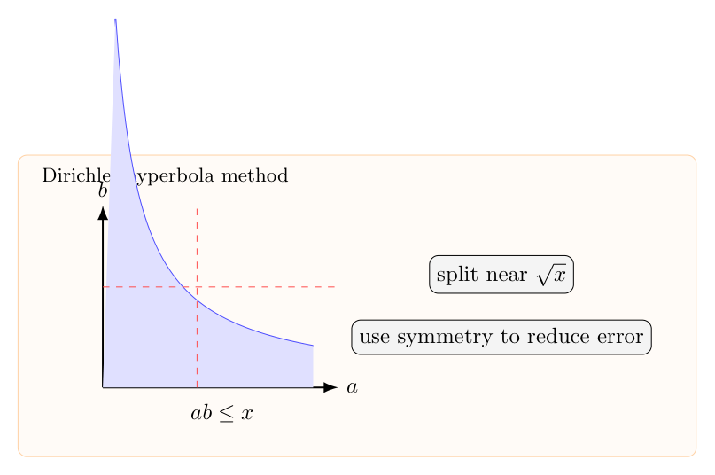
 , which is too big. But fortunately we can use the symmetry of hyperbola to improve the error term.
![\displaystyle \begin{array}{rcl} \sum_{1\leq n\leq x}d(n) & = & \sum_{ab\leq x}1\\ & = & \sum_{a\geq \sqrt{x}}[\frac{x}{b}]+\sum_{b\geq \sqrt{x}}[\frac{x}{a}]-\sum_{1\leq a,b\leq \sqrt{x}}1\\ & = & xlogx+(2\gamma-1)x+O(\sqrt{x}) \end{array}](https://s0.wp.com/latex.php?latex=%5Cdisplaystyle+%5Cbegin%7Barray%7D%7Brcl%7D+%5Csum_%7B1%5Cleq+n%5Cleq+x%7Dd%28n%29+%26+%3D+%26+%5Csum_%7Bab%5Cleq+x%7D1%5C%5C+%26+%3D+%26+%5Csum_%7Ba%5Cgeq+%5Csqrt%7Bx%7D%7D%5B%5Cfrac%7Bx%7D%7Bb%7D%5D%2B%5Csum_%7Bb%5Cgeq+%5Csqrt%7Bx%7D%7D%5B%5Cfrac%7Bx%7D%7Ba%7D%5D-%5Csum_%7B1%5Cleq+a%2Cb%5Cleq+%5Csqrt%7Bx%7D%7D1%5C%5C+%26+%3D+%26+xlogx%2B%282%5Cgamma-1%29x%2BO%28%5Csqrt%7Bx%7D%29+%5Cend%7Barray%7D+&bg=ffffff&fg=000000&s=0&c=20201002)


 denotes a polynomial of degree
  with leading term
  .
. is the residue of
  at
at  .
. ![\displaystyle \sum_{1\leq xy\leq n}[\frac{n}{xy}]=xP_2(logx)+O(x^{1-\frac{1}{3}+\epsilon}) \ \ \ \ \ (5)](https://s0.wp.com/latex.php?latex=%5Cdisplaystyle+%5Csum_%7B1%5Cleq+xy%5Cleq+n%7D%5B%5Cfrac%7Bn%7D%7Bxy%7D%5D%3DxP_2%28logx%29%2BO%28x%5E%7B1-%5Cfrac%7B1%7D%7B3%7D%2B%5Cepsilon%7D%29+%5C+%5C+%5C+%5C+%5C+%285%29&bg=ffffff&fg=000000&s=0&c=20201002)
![\displaystyle \sum_{1\leq xy\leq n}[\frac{n}{xy}]=\sum_{xyz\leq n}1 \ \ \ \ \ (6)](https://s0.wp.com/latex.php?latex=%5Cdisplaystyle+%5Csum_%7B1%5Cleq+xy%5Cleq+n%7D%5B%5Cfrac%7Bn%7D%7Bxy%7D%5D%3D%5Csum_%7Bxyz%5Cleq+n%7D1+%5C+%5C+%5C+%5C+%5C+%286%29&bg=ffffff&fg=000000&s=0&c=20201002)
![{([n^{\frac{1}{3}}],[n^{\frac{1}{3}}],[n^{\frac{1}{3}}])}](https://s0.wp.com/latex.php?latex=%7B%28%5Bn%5E%7B%5Cfrac%7B1%7D%7B3%7D%7D%5D%2C%5Bn%5E%7B%5Cfrac%7B1%7D%7B3%7D%7D%5D%2C%5Bn%5E%7B%5Cfrac%7B1%7D%7B3%7D%7D%5D%29%7D&bg=ffffff&fg=000000&s=0&c=20201002) is the central point under the hyperbola.
is the central point under the hyperbola.![{A_x=\sum_{1\leq r\leq [n^{\frac{1}{3}}]}\sum_{1\leq yz\leq [n^{\frac{2}{3}}]}[\frac{r}{yz}]}](https://s0.wp.com/latex.php?latex=%7BA_x%3D%5Csum_%7B1%5Cleq+r%5Cleq+%5Bn%5E%7B%5Cfrac%7B1%7D%7B3%7D%7D%5D%7D%5Csum_%7B1%5Cleq+yz%5Cleq+%5Bn%5E%7B%5Cfrac%7B2%7D%7B3%7D%7D%5D%7D%5B%5Cfrac%7Br%7D%7Byz%7D%5D%7D&bg=ffffff&fg=000000&s=0&c=20201002) .
.![{A_y=\sum_{1\leq r\leq [n^{\frac{1}{3}}]}\sum_{1\leq xz\leq [n^{\frac{2}{3}}]}[\frac{r}{yz}]}](https://s0.wp.com/latex.php?latex=%7BA_y%3D%5Csum_%7B1%5Cleq+r%5Cleq+%5Bn%5E%7B%5Cfrac%7B1%7D%7B3%7D%7D%5D%7D%5Csum_%7B1%5Cleq+xz%5Cleq+%5Bn%5E%7B%5Cfrac%7B2%7D%7B3%7D%7D%5D%7D%5B%5Cfrac%7Br%7D%7Byz%7D%5D%7D&bg=ffffff&fg=000000&s=0&c=20201002) .
.![{A_z=\sum_{1\leq r\leq [n^{\frac{1}{3}}]}\sum_{1\leq xy\leq [n^{\frac{2}{3}}]}[\frac{r}{yz}]}](https://s0.wp.com/latex.php?latex=%7BA_z%3D%5Csum_%7B1%5Cleq+r%5Cleq+%5Bn%5E%7B%5Cfrac%7B1%7D%7B3%7D%7D%5D%7D%5Csum_%7B1%5Cleq+xy%5Cleq+%5Bn%5E%7B%5Cfrac%7B2%7D%7B3%7D%7D%5D%7D%5B%5Cfrac%7Br%7D%7Byz%7D%5D%7D&bg=ffffff&fg=000000&s=0&c=20201002) .
.
![{\sum_{1\leq yz\leq [n^{\frac{2}{3}}]}[\frac{r}{yz}]}](https://s0.wp.com/latex.php?latex=%7B%5Csum_%7B1%5Cleq+yz%5Cleq+%5Bn%5E%7B%5Cfrac%7B2%7D%7B3%7D%7D%5D%7D%5B%5Cfrac%7Br%7D%7Byz%7D%5D%7D&bg=ffffff&fg=000000&s=0&c=20201002) and then integral it. This end the proof. For general
and then integral it. This end the proof. For general  , the story is the same, by induction.
 and use the Fubini theorem to calculate
  .
. 

 , it is known that
  is not right.
 , is there a asymptotic formula for
  ?
? is a polynomial with degree
  ?
? is a polynomial with degree
  ?
?
![\displaystyle \begin{array}{rcl} \frac{\{\frac{kn}{1}\}+\{\frac{kn}{2}\}+...+\{\frac{kn}{n}\}}{n} & = & \frac{\sum_{i=1}^k\frac{kn}{i}-\sum_{i=1}^n[\frac{kn}{i}]}{n}\\ & = & k(lnn+\gamma +\epsilon_n)-\frac{\sum_{i=1}^{kn}[\frac{kn}{i}]-\sum_{i=n+1}^{kn}[\frac{kn}{i}]}{n} \end{array}](https://s0.wp.com/latex.php?latex=%5Cdisplaystyle+%5Cbegin%7Barray%7D%7Brcl%7D+%5Cfrac%7B%5C%7B%5Cfrac%7Bkn%7D%7B1%7D%5C%7D%2B%5C%7B%5Cfrac%7Bkn%7D%7B2%7D%5C%7D%2B...%2B%5C%7B%5Cfrac%7Bkn%7D%7Bn%7D%5C%7D%7D%7Bn%7D+%26+%3D+%26+%5Cfrac%7B%5Csum_%7Bi%3D1%7D%5Ek%5Cfrac%7Bkn%7D%7Bi%7D-%5Csum_%7Bi%3D1%7D%5En%5B%5Cfrac%7Bkn%7D%7Bi%7D%5D%7D%7Bn%7D%5C%5C+%26+%3D+%26+k%28lnn%2B%5Cgamma+%2B%5Cepsilon_n%29-%5Cfrac%7B%5Csum_%7Bi%3D1%7D%5E%7Bkn%7D%5B%5Cfrac%7Bkn%7D%7Bi%7D%5D-%5Csum_%7Bi%3Dn%2B1%7D%5E%7Bkn%7D%5B%5Cfrac%7Bkn%7D%7Bi%7D%5D%7D%7Bn%7D+%5Cend%7Barray%7D+&bg=ffffff&fg=000000&s=0&c=20201002)
![\displaystyle S_k(n)=\sum_{i=1}^{kn}[\frac{kn}{i}]-\sum_{i=n+1}^{kn}[\frac{kn}{i}] \ \ \ \ \ (10)](https://s0.wp.com/latex.php?latex=%5Cdisplaystyle+S_k%28n%29%3D%5Csum_%7Bi%3D1%7D%5E%7Bkn%7D%5B%5Cfrac%7Bkn%7D%7Bi%7D%5D-%5Csum_%7Bi%3Dn%2B1%7D%5E%7Bkn%7D%5B%5Cfrac%7Bkn%7D%7Bi%7D%5D+%5C+%5C+%5C+%5C+%5C+%2810%29&bg=ffffff&fg=000000&s=0&c=20201002)
![\displaystyle \begin{array}{rcl} S_k(n) & = & (2\sum_{i=1}^{[\sqrt{kn}]}[\frac{kn}{i}]-[\sqrt{kn}]^2)-(\sum_{i=1}^k[\frac{kn}{i}]-kn)\\ & = & 2\sum_{i=1}^{[\sqrt{kn}]}\frac{kn}{i}-\sum_{i=1}^k\frac{kn}{i}+2\{\sqrt{kn}\}[\sqrt{kn}]+\{\sqrt{kn}\}^2-2\sum_{i=1}^{[\sqrt{kn}]}\{\frac{kn}{i}\}+\sum_{i=1}^k\{\frac{kn}{i}\}\\ & = & 2kn(ln[\sqrt{kn}]+\gamma+\epsilon_{[\sqrt{kn}]})-kn\sum_{i=1}^k\frac{1}{i}+r(n)\\ & = & knln(kn)+kn(2\gamma-\sum_{i=1}^k\frac{1}{i})+r'(n)\\ & = & knln n+kn(2\gamma+lnk-\sum_{i=1}^k\frac{1}{i})+r'(n) \end{array}](https://s0.wp.com/latex.php?latex=%5Cdisplaystyle+%5Cbegin%7Barray%7D%7Brcl%7D+S_k%28n%29+%26+%3D+%26+%282%5Csum_%7Bi%3D1%7D%5E%7B%5B%5Csqrt%7Bkn%7D%5D%7D%5B%5Cfrac%7Bkn%7D%7Bi%7D%5D-%5B%5Csqrt%7Bkn%7D%5D%5E2%29-%28%5Csum_%7Bi%3D1%7D%5Ek%5B%5Cfrac%7Bkn%7D%7Bi%7D%5D-kn%29%5C%5C+%26+%3D+%26+2%5Csum_%7Bi%3D1%7D%5E%7B%5B%5Csqrt%7Bkn%7D%5D%7D%5Cfrac%7Bkn%7D%7Bi%7D-%5Csum_%7Bi%3D1%7D%5Ek%5Cfrac%7Bkn%7D%7Bi%7D%2B2%5C%7B%5Csqrt%7Bkn%7D%5C%7D%5B%5Csqrt%7Bkn%7D%5D%2B%5C%7B%5Csqrt%7Bkn%7D%5C%7D%5E2-2%5Csum_%7Bi%3D1%7D%5E%7B%5B%5Csqrt%7Bkn%7D%5D%7D%5C%7B%5Cfrac%7Bkn%7D%7Bi%7D%5C%7D%2B%5Csum_%7Bi%3D1%7D%5Ek%5C%7B%5Cfrac%7Bkn%7D%7Bi%7D%5C%7D%5C%5C+%26+%3D+%26+2kn%28ln%5B%5Csqrt%7Bkn%7D%5D%2B%5Cgamma%2B%5Cepsilon_%7B%5B%5Csqrt%7Bkn%7D%5D%7D%29-kn%5Csum_%7Bi%3D1%7D%5Ek%5Cfrac%7B1%7D%7Bi%7D%2Br%28n%29%5C%5C+%26+%3D+%26+knln%28kn%29%2Bkn%282%5Cgamma-%5Csum_%7Bi%3D1%7D%5Ek%5Cfrac%7B1%7D%7Bi%7D%29%2Br%27%28n%29%5C%5C+%26+%3D+%26+knln+n%2Bkn%282%5Cgamma%2Blnk-%5Csum_%7Bi%3D1%7D%5Ek%5Cfrac%7B1%7D%7Bi%7D%29%2Br%27%28n%29+%5Cend%7Barray%7D+&bg=ffffff&fg=000000&s=0&c=20201002)
 ,
,  .
.

 , by combining the theorem

 is the volume of the unit ball in
  . Langrange proved that every natural number can be represented as the sum of four squares, i.e.
  , and Jacobi established the exact formula for the number of representations

 as the additive convolution of
  and
and  , i.e.
 squares by integration.
 in
in  ), indeed for
  we have
  if
if  is odd by the Jacobi formula. The only case of the lattice point problem for a ball which is not yet solved (i.e. the best possible error terms are not yet established) are for the circle(
 ) and the sphere (
 ).
). 
![{f(x)\in {\mathbb Z}[x]}](https://s0.wp.com/latex.php?latex=%7Bf%28x%29%5Cin+%7B%5Cmathbb+Z%7D%5Bx%5D%7D&bg=ffffff&fg=000000&s=0&c=20201002) is a irreducible polynomial. And for each prime
is a irreducible polynomial. And for each prime  , let
, let
 .
. 


 . We know
  is solvable iff
  or
or  . One side is easy, just by Fermat little theorem, the other hand need Fermat descent procedure, which of course could be done by Willson theorem. In this case,
 be an algebraic number field, i.e. the finite field extension of rational numbers, let
 ![\displaystyle \mathcal{O}_K=\{\alpha\in K, \alpha \ satisfied \ a\ monic \ polynomial\ in\ {\mathbb Z}[x]\} \ \ \ \ \ (23)](https://s0.wp.com/latex.php?latex=%5Cdisplaystyle+%5Cmathcal%7BO%7D_K%3D%5C%7B%5Calpha%5Cin+K%2C+%5Calpha+%5C+satisfied+%5C+a%5C+monic+%5C+polynomial%5C+in%5C+%7B%5Cmathbb+Z%7D%5Bx%5D%5C%7D+%5C+%5C+%5C+%5C+%5C+%2823%29&bg=ffffff&fg=000000&s=0&c=20201002)
 is a ring, we call it the ring of integer of
  uniquely.
 in
in ![{[\mathcal{O}_K:I]<\infty}](https://s0.wp.com/latex.php?latex=%7B%5B%5Cmathcal%7BO%7D_K%3AI%5D%3C%5Cinfty%7D&bg=ffffff&fg=000000&s=0&c=20201002) , and we can define the norm induce by index.
, and we can define the norm induce by index.
![\displaystyle N(I):=[\mathcal{O}_K:I] \ \ \ \ \ (24)](https://s0.wp.com/latex.php?latex=%5Cdisplaystyle+N%28I%29%3A%3D%5B%5Cmathcal%7BO%7D_K%3AI%5D+%5C+%5C+%5C+%5C+%5C+%2824%29&bg=ffffff&fg=000000&s=0&c=20201002)
 .
.
 , does the exist a asymptotic formula,

 is different prime ideal in
  ? For the question, there is a satisfied answer.
 is some algebraic number, which’s minor polynomial
  , factorize it in the polynomial ring
 ![{{\mathbb Z}_p[x]}](https://s0.wp.com/latex.php?latex=%7B%7B%5Cmathbb+Z%7D_p%5Bx%5D%7D&bg=ffffff&fg=000000&s=0&c=20201002) ,
,
 . Then apart from finite many primes, we have,
 .
. of ideals of
  equal to,
![\displaystyle \rho_k(X)+O(x^{1-\frac{1}{d}}), where \ d=[K:Q] \ \ \ \ \ (31)](https://s0.wp.com/latex.php?latex=%5Cdisplaystyle+%5Crho_k%28X%29%2BO%28x%5E%7B1-%5Cfrac%7B1%7D%7Bd%7D%7D%29%2C+where+%5C+d%3D%5BK%3AQ%5D+%5C+%5C+%5C+%5C+%5C+%2831%29&bg=ffffff&fg=000000&s=0&c=20201002)
 come from a determination systems
  , where
  ,
,  . The correlation of it and the Liuvillou function is 0, i.e. they are orthongonal to each other, more preseicesly it is just to say,
 should be randomness.
 ,
,  is a inrational, then the obersevation come from
  is orthogonal to Mobius function. due to
  is a basis of
  , suffice to proof,
 , and proof that the theorem MR hold we need only to proof it hold for
 ![{S\cap [1,2,...,n]}](https://s0.wp.com/latex.php?latex=%7BS%5Ccap+%5B1%2C2%2C...%2Cn%5D%7D&bg=ffffff&fg=000000&s=0&c=20201002) instead of
instead of ![{[1,2,...,n]}](https://s0.wp.com/latex.php?latex=%7B%5B1%2C2%2C...%2Cn%5D%7D&bg=ffffff&fg=000000&s=0&c=20201002)
 we have:
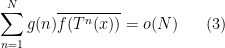
 .
. 
 . We can not get good estimate for all term,

![\displaystyle \begin{array}{rcl} |\sum_{p\in W}\sum_{n\in V}F(pn)g(pn)| & \leq & \sum_{n\in V}|g(n)|\cdot |\sum_{p\in W}F(pn)g(p)| \\ & \leq &\sum_{n\in V}|\sum_{p \in W}F(pn)g(p)|\\ & \overset{Cauchy-Schwarz}\leq & |V|^{\frac{1}{2}}[\sum_{n\in V}|\sum_{p\in W}F(pn)g(p)|^2]^{\frac{1}{2}}\\ & = & |V|^{\frac{1}{2}}[\sum_{p_1,p_2\in W}\sum_{n\in V}F(p_1n)\overline{F(p_2n)}g(p_1)\overline{g(p_2)}]^{\frac{1}{2}}\\ \end{array}](https://s0.wp.com/latex.php?latex=%5Cdisplaystyle+%5Cbegin%7Barray%7D%7Brcl%7D+%7C%5Csum_%7Bp%5Cin+W%7D%5Csum_%7Bn%5Cin+V%7DF%28pn%29g%28pn%29%7C+%26+%5Cleq+%26+%5Csum_%7Bn%5Cin+V%7D%7Cg%28n%29%7C%5Ccdot+%7C%5Csum_%7Bp%5Cin+W%7DF%28pn%29g%28p%29%7C+%5C%5C+%26+%5Cleq+%26%5Csum_%7Bn%5Cin+V%7D%7C%5Csum_%7Bp+%5Cin+W%7DF%28pn%29g%28p%29%7C%5C%5C+%26+%5Coverset%7BCauchy-Schwarz%7D%5Cleq+%26+%7CV%7C%5E%7B%5Cfrac%7B1%7D%7B2%7D%7D%5B%5Csum_%7Bn%5Cin+V%7D%7C%5Csum_%7Bp%5Cin+W%7DF%28pn%29g%28p%29%7C%5E2%5D%5E%7B%5Cfrac%7B1%7D%7B2%7D%7D%5C%5C+%26+%3D+%26+%7CV%7C%5E%7B%5Cfrac%7B1%7D%7B2%7D%7D%5B%5Csum_%7Bp_1%2Cp_2%5Cin+W%7D%5Csum_%7Bn%5Cin+V%7DF%28p_1n%29%5Coverline%7BF%28p_2n%29%7Dg%28p_1%29%5Coverline%7Bg%28p_2%29%7D%5D%5E%7B%5Cfrac%7B1%7D%7B2%7D%7D%5C%5C+%5Cend%7Barray%7D+&bg=ffffff&fg=000000&s=0&c=20201002)
![\displaystyle |V|^{\frac{1}{2}}[\sum_{p_1\neq p_2\in W}\sum_{n\in V}F(p_1n)\overline{F(p_2n)}g(p_1)\overline{g(p_2)}]^{\frac{1}{2}}+|V|^{\frac{1}{2}}[\sum_{p\in W}\sum_{n\in V}|F(pn)|^2]^{\frac{1}{2}} \ \ \ \ \ (7)](https://s0.wp.com/latex.php?latex=%5Cdisplaystyle+%7CV%7C%5E%7B%5Cfrac%7B1%7D%7B2%7D%7D%5B%5Csum_%7Bp_1%5Cneq+p_2%5Cin+W%7D%5Csum_%7Bn%5Cin+V%7DF%28p_1n%29%5Coverline%7BF%28p_2n%29%7Dg%28p_1%29%5Coverline%7Bg%28p_2%29%7D%5D%5E%7B%5Cfrac%7B1%7D%7B2%7D%7D%2B%7CV%7C%5E%7B%5Cfrac%7B1%7D%7B2%7D%7D%5B%5Csum_%7Bp%5Cin+W%7D%5Csum_%7Bn%5Cin+V%7D%7CF%28pn%29%7C%5E2%5D%5E%7B%5Cfrac%7B1%7D%7B2%7D%7D+%5C+%5C+%5C+%5C+%5C+%287%29&bg=ffffff&fg=000000&s=0&c=20201002)
![\displaystyle |V|^{\frac{1}{2}}[\sum_{p_1\neq p_2\in W}\sum_{n\in V}F(p_1n)\overline{F(p_2n)}g(p_1)\overline{g(p_2)}]^{\frac{1}{2}} =o(|W||V|) \ \ \ \ \ (8)](https://s0.wp.com/latex.php?latex=%5Cdisplaystyle+%7CV%7C%5E%7B%5Cfrac%7B1%7D%7B2%7D%7D%5B%5Csum_%7Bp_1%5Cneq+p_2%5Cin+W%7D%5Csum_%7Bn%5Cin+V%7DF%28p_1n%29%5Coverline%7BF%28p_2n%29%7Dg%28p_1%29%5Coverline%7Bg%28p_2%29%7D%5D%5E%7B%5Cfrac%7B1%7D%7B2%7D%7D+%3Do%28%7CW%7C%7CV%7C%29+%5C+%5C+%5C+%5C+%5C+%288%29&bg=ffffff&fg=000000&s=0&c=20201002)

![\displaystyle |V|^{\frac{1}{2}}[\sum_{p\in W}\sum_{n\in V}|F(pn)|^2]^{\frac{1}{2}}=o(|W||V|) \ \ \ \ \ (10)](https://s0.wp.com/latex.php?latex=%5Cdisplaystyle+%7CV%7C%5E%7B%5Cfrac%7B1%7D%7B2%7D%7D%5B%5Csum_%7Bp%5Cin+W%7D%5Csum_%7Bn%5Cin+V%7D%7CF%28pn%29%7C%5E2%5D%5E%7B%5Cfrac%7B1%7D%7B2%7D%7D%3Do%28%7CW%7C%7CV%7C%29+%5C+%5C+%5C+%5C+%5C+%2810%29&bg=ffffff&fg=000000&s=0&c=20201002)
 and trivial inequality
 and then break up
  into
into  , this mean,

 in
in  , if
, if  ,
,  is uniformly distributed, then
 : Given
  ,
,  coverages to a uniformly distribution in
  as
as  .
. .
. 


 when
when  , one has:
 .
.
 norm, by Chebyschev inequality, this could be control by
  norm, so we only need to establish the following,

![{[xe^{-\frac{1}{T}},xe^{\frac{1}{T}}]\sim [x-H,x+H]}](https://s0.wp.com/latex.php?latex=%7B%5Bxe%5E%7B-%5Cfrac%7B1%7D%7BT%7D%7D%2Cxe%5E%7B%5Cfrac%7B1%7D%7BT%7D%7D%5D%5Csim+%5Bx-H%2Cx%2BH%5D%7D&bg=ffffff&fg=000000&s=0&c=20201002) .
. and
and  is to make that
  .
.

 . Note that,




 with additive structure, it could be looked as a lots of wave with the periodic given by primes, so we could do a orthogonal decomposition in the fractional space, try to prove the cutoff is a error term and we get such a monotonically inequality.
 , we have Euler-product formula:
 leads to following result:
 , but take average at a area which is natural generated and compatible with multiplication, this identity carry a lot of information of the multiplicative property. Which is crucial to get a good estimate for the quality we consider about.
 which is carefully chosen. And we do not consider [X,2X] with linear structure anymore , instead reconsider the decomposition:
![{[X,2X]=\amalg_{i=1}^n (I_i\times J_i) \amalg U}](https://s0.wp.com/latex.php?latex=%7B%5BX%2C2X%5D%3D%5Camalg_%7Bi%3D1%7D%5En+%28I_i%5Ctimes+J_i%29+%5Camalg+U%7D&bg=ffffff&fg=000000&s=0&c=20201002)
 it equipped with a bilinear structure. And
  is a very small set,
  which is in fact have much better estimate.




 as
as  ,
,![\displaystyle \Omega^m=\{a_mx^m+a_{m-1}x^{m-1}+...+a_1x+a_0 | a_m,...,a_1,a_0\in [0,1]\}](https://s0.wp.com/latex.php?latex=%5Cdisplaystyle+%5COmega%5Em%3D%5C%7Ba_mx%5Em%2Ba_%7Bm-1%7Dx%5E%7Bm-1%7D%2B...%2Ba_1x%2Ba_0+%7C+a_m%2C...%2Ca_1%2Ca_0%5Cin+%5B0%2C1%5D%5C%7D&bg=ffffff&fg=000000&s=0&c=20201002)
 is a multiplicative function, i.e.
  .
. 
 is a polynomial function then we have the following result,
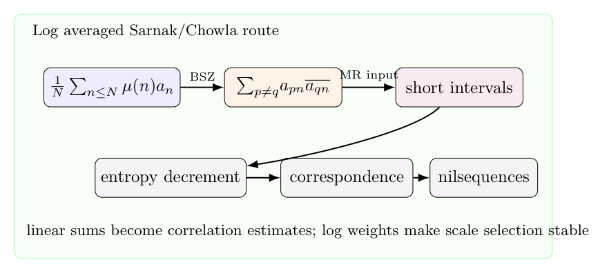

 . But by stupid use Cauchy we get following,

 . But this is still difficult to estimate, merely because of we need to control the variation of convolution of
  with itself on
  .
. be finitely supported functions obeying the orthonormality relationship,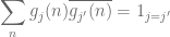
 . Then for any function
  , we have,
 .
. to be a orthogonal basis on
  , then this inequality is a natural corollary.
 be a non-negative function. Let
  vanishes whenever
  vanishes, we have
 of complex numbers with
  , with the convention that
  vanishes whenever
  both vanish.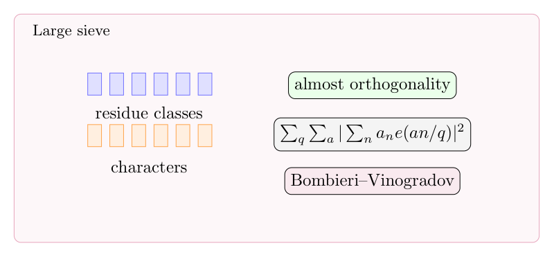
 when
when  , one has:
 for almost all
  .
. norms of the quality we wish to charge. It is just trying to understanding


 ) with additive structure, it could be looked as a lots of wave with the periodic given by primes, so we could do a orthogonal decomposition in the fractional space, try to prove the cutoff is a error term and we get such a monotonically inequality.
 , we have Euler-product formula:
 leads to following result:
 , but take average at a area which is natural generated and compatible with multiplication, this identity carry a lot of information of the multiplicative property. Which is crucial to get a good estimate for the quality we consider about.
 , but use several sets
  which is carefully chosen. And we do not consider [X,2X] with linear structure anymore , instead reconsider the decomposition:
![[X,2X]=\amalg_{i=1}^n (I_i\times J_i) \amalg U](https://s0.wp.com/latex.php?latex=%5BX%2C2X%5D%3D%5Camalg_%7Bi%3D1%7D%5En+%28I_i%5Ctimes+J_i%29+%5Camalg+U&bg=ffffff&fg=5e5e5e&s=0&c=20201002)
 it equipped with a bilinear structure. And
  is a very small set, $|U|=o(X)$ which is in fact have much better estimate.

 is irrational and
  .
. , this could view as a effective uniformly distribute result of dynamic system:
 ![([0,1]^n,T)](https://s0.wp.com/latex.php?latex=%28%5B0%2C1%5D%5En%2CT%29&bg=ffffff&fg=5e5e5e&s=0&c=20201002) , where
, where  ,
,  is a nilpotent matrix, matrix
  is identity but with a irrational number
  elements.
 , we could do this approach with the last
  , which will corresponding to
  , i.e. we could apply the “rigid trick” to prove sequences
  is uniformly distribute according to
  .
. .
. .
. which is roughly the same). That is just the orbits
  have quasi-period property, that is to say, under certain norms, it could be understand as the limits of periodic sequences. So it is natural to approximation
 is just the periodic approximation sequence which come from the best approximation (critical point of
  ), which natural occur in continue fractional. And by this we already arrive a non qualitative form result of
  with
with  .
. case. The reason of this result could be true is just because the natural estimate for the best approximation of
 :
: and is critical to observe that the progression of difference structure in it. The goal of this approach is to establish some result from the finite torsion structure(multilinear structure). That is to say, the boundary is high order thing in all direction but there is only one direction attend to infinity the other is just a finite torsion, and we wish to get more information from the extra structure.
 case:
case:
 be a entropy zero topological dynamic system. Let Mobius function be defined as
  , where $latex$ is the number of different primes occur in the decomposition of
  .
. and
and  , observable
  is orthogonal to the Mobius function; i.e. ,
 is the skew product on
![[0,1]](https://s0.wp.com/latex.php?latex=%5B0%2C1%5D&bg=ffffff&fg=5e5e5e&s=0&c=20201002) .
. ,
, :
:
 , where
  .
.
 is suffice large primes pair.
 on
on  and the general case
  where A is a upper-triangle matrix with diagonal 1; i.e.
  , B is nilpotent. So the sarnak conjecture in this case is reduce to the Davenport estimate on exponent by B-Z-S theorem:
 ,
,  .
. step by step and with a renormalization process to glue the neighbor rotations.
 , and it is easy to see there is only one case is nontrivial that is permutation:
  . We explain a little more with other trivial case:
 , the interval exchange map is just a rotation and for which the sarnak conjecture is just come from:
 ,
,  .
. .
. is a rotation on
  but it is a identity map on
  and the orbits of point only lying one of $I_1\cap I_2, I_3$, lying in which one depend on the original point
  we take is lying in which one.
 which are not the common endpoint of them. Then you get two circle glue like a “8” , and
  is just rotate one of it and make the other one to be invariance.
 .
. , then
 ![A\cap B=\emptyset, A\cup B=[0,1]](https://s0.wp.com/latex.php?latex=A%5Ccap+B%3D%5Cemptyset%2C+A%5Ccup+B%3D%5B0%2C1%5D&bg=ffffff&fg=5e5e5e&s=0&c=20201002) . And
. And  ,
,  . the rotation
  ,
,  .
.
 ,
, .
.
 ?
? , then by following clear calculate:
![\int_{[0,1]^k}|f_k(x,N)|^{2s}dx_1...dx_k =\int_{[0,1]^k}|\sum_{1\leq n\leq N}e(nx_1+n^2x_2+...+n^kx_k)|^{2s}dx_1dx_2...dx_k &=\int_{[0,1]^k}\sum_{1\leq n_1,...,n_{2s}\leq N}e^{2\pi i[(n_1+...+n_{2s})x_1+...+(n_1^k+...+n_{2s}^k)x_k-(n_{s+1}+...+n_{2s})x_1-...-(n_{s+1}^k+...+n_{2s}^k)x_k]} &=|\{(n_1,...,n_{2s})| n_1^j+...+n_s^j=n_{s+1}^j+...+n_{2s}^j,\forall 1\leq j\leq k\}|](https://s0.wp.com/latex.php?latex=%5Cint_%7B%5B0%2C1%5D%5Ek%7D%7Cf_k%28x%2CN%29%7C%5E%7B2s%7Ddx_1...dx_k+%3D%5Cint_%7B%5B0%2C1%5D%5Ek%7D%7C%5Csum_%7B1%5Cleq+n%5Cleq+N%7De%28nx_1%2Bn%5E2x_2%2B...%2Bn%5Ekx_k%29%7C%5E%7B2s%7Ddx_1dx_2...dx_k+%26%3D%5Cint_%7B%5B0%2C1%5D%5Ek%7D%5Csum_%7B1%5Cleq+n_1%2C...%2Cn_%7B2s%7D%5Cleq+N%7De%5E%7B2%5Cpi+i%5B%28n_1%2B...%2Bn_%7B2s%7D%29x_1%2B...%2B%28n_1%5Ek%2B...%2Bn_%7B2s%7D%5Ek%29x_k-%28n_%7Bs%2B1%7D%2B...%2Bn_%7B2s%7D%29x_1-...-%28n_%7Bs%2B1%7D%5Ek%2B...%2Bn_%7B2s%7D%5Ek%29x_k%5D%7D+%26%3D%7C%5C%7B%28n_1%2C...%2Cn_%7B2s%7D%29%7C+n_1%5Ej%2B...%2Bn_s%5Ej%3Dn_%7Bs%2B1%7D%5Ej%2B...%2Bn_%7B2s%7D%5Ej%2C%5Cforall+1%5Cleq+j%5Cleq+k%5C%7D%7C+&bg=ffffff&fg=5e5e5e&s=0&c=20201002)
![J_{s,k}(N)=\int_{[0,1]^k}|f_k(x,N)|^{2s}dx_1...dx_k](https://s0.wp.com/latex.php?latex=J_%7Bs%2Ck%7D%28N%29%3D%5Cint_%7B%5B0%2C1%5D%5Ek%7D%7Cf_k%28x%2CN%29%7C%5E%7B2s%7Ddx_1...dx_k+&bg=ffffff&fg=5e5e5e&s=0&c=20201002)
 ,we have:
![E_{[0,1]}(g)](https://s0.wp.com/latex.php?latex=E_%7B%5B0%2C1%5D%7D%28g%29&bg=ffffff&fg=5e5e5e&s=0&c=20201002) cut off $E_{[0,1]}(g)$ into a lot of small boxes
cut off $E_{[0,1]}(g)$ into a lot of small boxes  , then the $L_{d(d+1)})$ norms of the operator could be bounded very well, in fact it is near orthonagonal.
 ,$0<\delta\leq 1$. Then for each ball
  of radious at least
  .
.![||E_{[0,1]}g||_{L^{d(d+1)}(w_B)}<< \delta^{-\epsilon}(\sum_{J\subset [0,1],|J|=\delta}||E_Jg||^2_{L^{d(d+1)(w_B)}})^{\frac{1}{2}}](https://s0.wp.com/latex.php?latex=%7C%7CE_%7B%5B0%2C1%5D%7Dg%7C%7C_%7BL%5E%7Bd%28d%2B1%29%7D%28w_B%29%7D%3C%3C+%5Cdelta%5E%7B-%5Cepsilon%7D%28%5Csum_%7BJ%5Csubset+%5B0%2C1%5D%2C%7CJ%7C%3D%5Cdelta%7D%7C%7CE_Jg%7C%7C%5E2_%7BL%5E%7Bd%28d%2B1%29%28w_B%29%7D%7D%29%5E%7B%5Cfrac%7B1%7D%7B2%7D%7D&bg=ffffff&fg=5e5e5e&s=0&c=20201002)
 runs over a partition of
  -intervals)
![\int_{[0,1]^k}|\sum_{1\leq n\leq N}e(nx_1+n^2x_2+...+n^kx_k)|^{2s}dx_1dx_2...dx_n](https://s0.wp.com/latex.php?latex=%5Cint_%7B%5B0%2C1%5D%5Ek%7D%7C%5Csum_%7B1%5Cleq+n%5Cleq+N%7De%28nx_1%2Bn%5E2x_2%2B...%2Bn%5Ekx_k%29%7C%5E%7B2s%7Ddx_1dx_2...dx_n&bg=ffffff&fg=5e5e5e&s=0&c=20201002)
 norm of a constant function
  , with a lebergue measure
  on curve
  . this curve
  could be view as a canonical curve with non-vanish guess curvature.
 , then guess curvature of
  is a natural induced lebergue measure on
  come from rescaling arument.


 .
. ,especially
  .
. .
.

 .
. .
. .
. .(*)
.(*) constant.(after renormelization)
 of (*).
 ,
, .
. and
and  .
. .
. .
.
 中的可观测量是指
 ,$f\in C(T^2)$.
 ,由于
,由于 是
是 的一组基,只需对
 证明
证明 ,我们有\\
 \\
\\ \\
\\ \\
\\ \\
\\ \\
\\ :
:
 为多项式函数,我们有指数和估计:
 情形是引理的直接推论。接下来处理
 情形,这种情形下,我们定义
![\alpha=[q_1,q_2,q_3,....]](https://s0.wp.com/latex.php?latex=%5Calpha%3D%5Bq_1%2Cq_2%2Cq_3%2C....%5D&bg=ffffff&fg=5e5e5e&s=0&c=20201002)
 ,
, 那么:
那么:


 是一个质数,对于
 :\\定义
:\\定义 , 定义
, 定义 满足:\\
满足:\\ 的一段区间$I$,对任意
 ,
,

 \\
\\ 是Mobius函数
 和
和 做cut off来简化问题。\\
 ,则
,则 .
. ,则根据分部积分公式
 .\\
.\\

 时,我们可以找到
 当$N\to \infty$,使得
 的部分可以被cut off.
 关于
关于
![r_i \in [0,q_{i}-1]](https://s0.wp.com/latex.php?latex=r_i+%5Cin+%5B0%2Cq_%7Bi%7D-1%5D+&bg=ffffff&fg=5e5e5e&s=0&c=20201002)
 不为0,为什么要利用Ostrowoski表示,关键在于Ostrowoski表示中的标架
 是最佳逼近下最好的标架。\\
 标准长度
标准长度 如下:
如下:![l_1=\alpha,l_{k+1}=1-[\frac{1}{l_k}]l_k](https://s0.wp.com/latex.php?latex=l_1%3D%5Calpha%2Cl_%7Bk%2B1%7D%3D1-%5B%5Cfrac%7B1%7D%7Bl_k%7D%5Dl_k&bg=ffffff&fg=5e5e5e&s=0&c=20201002)
 ,做一些微小的计算会发现第k个

 在这个区间中的均匀分布性的余项可以得到很好地控制。
 ,对任意长度为
 的区间
的区间 ,
, 我们有:
我们有:
 提升为
提升为 ,因为实轴上长度为
 中的元素,有由于长度为
 的区间中有
的区间中有![[n\alpha]](https://s0.wp.com/latex.php?latex=%5Bn%5Calpha%5D&bg=ffffff&fg=5e5e5e&s=0&c=20201002) 个整数,所以:
个整数,所以:![\sum_{n=1}^N\chi_{(a,b)}(\{n\alpha\})=[N\alpha]=N(b-a)+O(1)](https://s0.wp.com/latex.php?latex=%5Csum_%7Bn%3D1%7D%5EN%5Cchi_%7B%28a%2Cb%29%7D%28%5C%7Bn%5Calpha%5C%7D%29%3D%5BN%5Calpha%5D%3DN%28b-a%29%2BO%281%29&bg=ffffff&fg=5e5e5e&s=0&c=20201002)