旧博客原文
原题:Log average sarnak conjecture
This is a note concentrate on the log average Sarnak conjecture, after the work of Matomaki and Raziwill on the estimate of multiplication function of short interval. Given a overview of the presented tools and method dealing with this conjectue.
1. Introduction
Sarnak conjecture \cite{Sarnak} assert that for any obersevable 



This is a very natural raised conjecture, Liuville function is the presentation of primes, due to we always believe the distribution of primes in 
It has been known as observed by Landau \cite{Laudau} that the simplest case,

already equivalent to the prime number theorem. It is not difficult to deduce the spetial case of Sarnak conjecture when with the obersevation in $latex {(1)}&fg=000000$ come from finite dynamic system is equivalent to the prime number theorem in athremetic progress by the similar argument. Besides this two classical result, may be the first new result was established by Davenport,
Theorem 1 Let
,
is a inrational, then the obersevation come from
is orthogonal to Mobius function. due to
is a basis of
, suffice to proof,

There is a lots of spetial situations of Sarnak’s conjecture have been established, The parts I mainly cared is the following:
- Interval exchange map.
- Skew product flow.
- Obersevable come from One dimensional zero entropy flow.
- Nilsequences.
But in this note, I do not want to explain the tecnical and tools to establish this result, but considering an equivalent conjecture of Sarnak conjecture, named Chowla conjecture, and explain the underlying insight of the suitable weak statement, i.e. the log average Chowla conjecture and the underlying insight of it.
The note is organized as following way, in the next section $latex {(2)}&fg=000000$, we give a self-contained introduction on the tools called Bourgain-Sarnak-Ziegler critation, explain the relationship of this critation and the sum-product phenomenon, also given some more general critation along the philosephy use in establish the Bourgain-Sarnak-Ziegler critation, which maybe useful in following development combine with some other tools. The key point is transform the sum from linear sum to bilinear sum and decomposition the bilinear sum into diagonal part and off-diagonal part, use the assume in the critation to argue the off-diagonal part is small and on the orther hand the diagonal part is also small by the trivial estimate and the volume of diogonal is small, this is very similar to a suitable Caderon-Zugmund decomposition.
In section $latex {(4)}&fg=000000$, I try to give a proof sketch of the result of Matomaki and Raziwill, which is also a key tools to understanding the Sarnak conjecture, or equivalent the Chowla conjecture. The key points of the proof contains following:
- Find a suitable fourier indentity
- Construct a multiplication-addition dense subset
, and proof that the theorem MR hold we need only to proof it hold for
instead of
- Involve the power of euler product formula. divide the whole interval into a lot of small interval with smaller and smaller scale and a residue part. We look the part come from every small scale as a major term and look the residue part as minor term.
- Deal with the major term at every scale, by a combitorios identity and second moments method.
- find a enough decay estimate from a scale to the next smaller scale.
- Deal with the minor term by the H… lemma.
![{[1,2,...,n]}](https://s0.wp.com/latex.php?latex=%7B%5B1%2C2%2C...%2Cn%5D%7D&bg=ffffff&fg=000000&s=0&c=20201002)
Due to the theorem of MR do not exausted the method they developed, we trying to make some more result with their method, Tao and Matomaki attain the average version of Chowla conjecture is true by this way, and combine this argument and the entropy decresment argument they established the 2 partten of the log average Chowla conjecture is true. Very recently Tao and his coperator proved the odd partten case of log average chowla conjecture is true, combine an argument of frustenberg crresponding principle and entopy decresment argument. But it seems the even and large than 2 case is much difficult and seems need something new to combine with the method of MR and entropy decresment and frunstenberg corresponfing principle to make some progress.
So, in section $latex {(5)}&fg=000000$, we give a self-contain introduction to the entropy decresment argument of Tao, and combine with the frustenberg corresponding principle.
In the last section $latex {(6)}&fg=000000$, I state some result and method and phylosphy of them I get on nilsequences and wish to combine them with the previous method to make some progress on log average Chowla conjecture on the even partten case.
\newpage
2. Bourgain-Sarnak-Zieglar creation
We begin with the easiest one, this is the main result established in \cite{BSZ}, I try to give the main ideal under the proof, but with a no quantitative version is the following,
Theorem 2 (Bourgain-Sarnak-Zieglar creation, not quantitative version) if for all primes
we have:
Then for multiplication function
we have

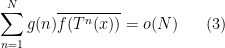
Remark 1 For simplify we identify
.
The idea is following, break the sum into a bilinear one, so, of course, we multiplication it with itself. i.e. we consider to control,
To control 4, we need exhausted the mutiplication property of
. We can not get good estimate for all term,
The condition in our hand if following,
So, just like the situation of Cotlar-Stein lemma \cite{Cotlar-Stein lemma}, we wish to estimate like following:
Then we consider divide the sum into diagonal part and non-diagonal part, as following,
But the first part is small, i.e.
Because of
and the second part is small, i.e.
Because diagonal part is small in
and trivial inequality



![\displaystyle \begin{array}{rcl} |\sum_{p\in W}\sum_{n\in V}F(pn)g(pn)| & \leq & \sum_{n\in V}|g(n)|\cdot |\sum_{p\in W}F(pn)g(p)| \\ & \leq &\sum_{n\in V}|\sum_{p \in W}F(pn)g(p)|\\ & \overset{Cauchy-Schwarz}\leq & |V|^{\frac{1}{2}}[\sum_{n\in V}|\sum_{p\in W}F(pn)g(p)|^2]^{\frac{1}{2}}\\ & = & |V|^{\frac{1}{2}}[\sum_{p_1,p_2\in W}\sum_{n\in V}F(p_1n)\overline{F(p_2n)}g(p_1)\overline{g(p_2)}]^{\frac{1}{2}}\\ \end{array}](https://s0.wp.com/latex.php?latex=%5Cdisplaystyle+%5Cbegin%7Barray%7D%7Brcl%7D+%7C%5Csum_%7Bp%5Cin+W%7D%5Csum_%7Bn%5Cin+V%7DF%28pn%29g%28pn%29%7C+%26+%5Cleq+%26+%5Csum_%7Bn%5Cin+V%7D%7Cg%28n%29%7C%5Ccdot+%7C%5Csum_%7Bp%5Cin+W%7DF%28pn%29g%28p%29%7C+%5C%5C+%26+%5Cleq+%26%5Csum_%7Bn%5Cin+V%7D%7C%5Csum_%7Bp+%5Cin+W%7DF%28pn%29g%28p%29%7C%5C%5C+%26+%5Coverset%7BCauchy-Schwarz%7D%5Cleq+%26+%7CV%7C%5E%7B%5Cfrac%7B1%7D%7B2%7D%7D%5B%5Csum_%7Bn%5Cin+V%7D%7C%5Csum_%7Bp%5Cin+W%7DF%28pn%29g%28p%29%7C%5E2%5D%5E%7B%5Cfrac%7B1%7D%7B2%7D%7D%5C%5C+%26+%3D+%26+%7CV%7C%5E%7B%5Cfrac%7B1%7D%7B2%7D%7D%5B%5Csum_%7Bp_1%2Cp_2%5Cin+W%7D%5Csum_%7Bn%5Cin+V%7DF%28p_1n%29%5Coverline%7BF%28p_2n%29%7Dg%28p_1%29%5Coverline%7Bg%28p_2%29%7D%5D%5E%7B%5Cfrac%7B1%7D%7B2%7D%7D%5C%5C+%5Cend%7Barray%7D+&bg=ffffff&fg=000000&s=0&c=20201002)
![\displaystyle |V|^{\frac{1}{2}}[\sum_{p_1\neq p_2\in W}\sum_{n\in V}F(p_1n)\overline{F(p_2n)}g(p_1)\overline{g(p_2)}]^{\frac{1}{2}}+|V|^{\frac{1}{2}}[\sum_{p\in W}\sum_{n\in V}|F(pn)|^2]^{\frac{1}{2}} \ \ \ \ \ (7)](https://s0.wp.com/latex.php?latex=%5Cdisplaystyle+%7CV%7C%5E%7B%5Cfrac%7B1%7D%7B2%7D%7D%5B%5Csum_%7Bp_1%5Cneq+p_2%5Cin+W%7D%5Csum_%7Bn%5Cin+V%7DF%28p_1n%29%5Coverline%7BF%28p_2n%29%7Dg%28p_1%29%5Coverline%7Bg%28p_2%29%7D%5D%5E%7B%5Cfrac%7B1%7D%7B2%7D%7D%2B%7CV%7C%5E%7B%5Cfrac%7B1%7D%7B2%7D%7D%5B%5Csum_%7Bp%5Cin+W%7D%5Csum_%7Bn%5Cin+V%7D%7CF%28pn%29%7C%5E2%5D%5E%7B%5Cfrac%7B1%7D%7B2%7D%7D+%5C+%5C+%5C+%5C+%5C+%287%29&bg=ffffff&fg=000000&s=0&c=20201002)
![\displaystyle |V|^{\frac{1}{2}}[\sum_{p_1\neq p_2\in W}\sum_{n\in V}F(p_1n)\overline{F(p_2n)}g(p_1)\overline{g(p_2)}]^{\frac{1}{2}} =o(|W||V|) \ \ \ \ \ (8)](https://s0.wp.com/latex.php?latex=%5Cdisplaystyle+%7CV%7C%5E%7B%5Cfrac%7B1%7D%7B2%7D%7D%5B%5Csum_%7Bp_1%5Cneq+p_2%5Cin+W%7D%5Csum_%7Bn%5Cin+V%7DF%28p_1n%29%5Coverline%7BF%28p_2n%29%7Dg%28p_1%29%5Coverline%7Bg%28p_2%29%7D%5D%5E%7B%5Cfrac%7B1%7D%7B2%7D%7D+%3Do%28%7CW%7C%7CV%7C%29+%5C+%5C+%5C+%5C+%5C+%288%29&bg=ffffff&fg=000000&s=0&c=20201002)

![\displaystyle |V|^{\frac{1}{2}}[\sum_{p\in W}\sum_{n\in V}|F(pn)|^2]^{\frac{1}{2}}=o(|W||V|) \ \ \ \ \ (10)](https://s0.wp.com/latex.php?latex=%5Cdisplaystyle+%7CV%7C%5E%7B%5Cfrac%7B1%7D%7B2%7D%7D%5B%5Csum_%7Bp%5Cin+W%7D%5Csum_%7Bn%5Cin+V%7D%7CF%28pn%29%7C%5E2%5D%5E%7B%5Cfrac%7B1%7D%7B2%7D%7D%3Do%28%7CW%7C%7CV%7C%29+%5C+%5C+%5C+%5C+%5C+%2810%29&bg=ffffff&fg=000000&s=0&c=20201002)

But the method in remark 2 is not always make sense in any situation, we need to construct two suitable sets 


But this
Theorem 3 (Prime number theorem)

Morally speaking, this is the statement that the primes, which is the generator of multiplication function, is not very sparse.
3. Van der curpurt trick
There is the statement of Van der carport theorem:
Theorem 4 (Van der curpurt trick) Given a sequences
in
, if
,
is uniformly distributed, then
I do not know how to establish this theorem with no extra condition, but this result is true at least for polynomial flow. \newpage Proof:


This type of trick could also establish the following result, which could be understand as a discretization of the Vinegradov lemma.
Remark 3
Uniformly distribution result of
: Given
,
coverages to a uniformly distribution in
as
.
Remark 4 But I definitely do not know how to establish the similar result when
.
Remark 5
This trick could also help to establish estimate of correlation of low complexity sequences and multiplicative function, such as result:
Maybe with the help of B-Z-S theorem.

\newpage
4. Matomaki and Raziwill’s work
In this section we explain the main idea underlying the paper \cite{KAISA MATOMA 虉KI AND MAKSYM RADZIWILL}. But play with a toy model, i.e. the corresponding corollary of the original result on Liouville鈥檚 function.
Definition 5 (Lioville’s function)

Remark 6
is equivalent to the prime number theorem 3.

The most important beakgrouth of analytic number theory is the new understanding of multiplication function on share interval, this result is established by Kaisa Matom盲ki and Maksym Radziwill. Two very young and intelligent superstars.
The main theorem in them article is :
Theorem 6 (Matomaki,Radziwill) As soon as
when
, one has:
for almost all
.

In my understanding of the result, the main strategy is:
- Parseval indetity, transform to Dirchelet polynomial.
- Involved by multiplication property, spectral decomposition.
- From linear to multilinear , Cauchy schwarz inequality.
- major term estimate.
- Estimate the contribution of area which is not filled.
4.1. Parseval indetity, transform to Dirchelet polynomial
We wish to establish the equality,

This is the 


We wish to transform from the discretization sum to a continue sum, that is,

Remark 7 There are two points to understand why 19 and 18 are the same.
.
and
is to make that
.
So the Magnitude of 18 and 19 are the same. i.e.

Now we try to transform 19 by Parseval indetity, this is something about the

Then 

So by Parseval identity, we have,

Remark 8 We know the Fejer kernel satisfied,

So morally speaking, we get the following identity.

In fact we do a cutoff, the quality we really consider is just:

established the monotonically inequality:
Theorem 7 (Paserval type identity)

Remark 9
In my understanding, This is a perspective of the quality, due to the quality is a multiplicative function integral on a domain
with additive structure, it could be looked as a lots of wave with the periodic given by primes, so we could do a orthogonal decomposition in the fractional space, try to prove the cutoff is a error term and we get such a monotonically inequality.
But at once we get the monotonically inequality, we could look it as a聽compactification process and this process still carry most of the information so lead to the inequality.
It seems something similar occur in the attack of the moments estimate of zeta function by the second author. And it is also could be looked as something similar to the 聽spectral decomposition with some basis come from multiplication generators, i.e. primes.
4.2. Involved by multiplication property, spectral decomposition
I called it is “spectral decomposition”, but this is not very exact. Anyway, the thing I want to say is that for multiplication function 

But anyway, we do not use the whole power of multiplication just use it on primes, i.e. 

This is a identity about the function 
4.3. From linear to multilinear , Cauchy schwarz
Now, we do not use one sets 

![{[X,2X]=\amalg_{i=1}^n (I_i\times J_i) \amalg U}](https://s0.wp.com/latex.php?latex=%7B%5BX%2C2X%5D%3D%5Camalg_%7Bi%3D1%7D%5En+%28I_i%5Ctimes+J_i%29+%5Camalg+U%7D&bg=ffffff&fg=000000&s=0&c=20201002)
On every 


Now we just use a Cauchy-Schwarz:

4.4. major term estimate


4.5. estimate the contribution of area which is not filled
\newpage
5. Entropy dcrement argument
\newpage
6. Correlation with nilsequences
I wish to establish the following estimate:

Where we have 

![\displaystyle \Omega^m=\{a_mx^m+a_{m-1}x^{m-1}+...+a_1x+a_0 | a_m,...,a_1,a_0\in [0,1]\}](https://s0.wp.com/latex.php?latex=%5Cdisplaystyle+%5COmega%5Em%3D%5C%7Ba_mx%5Em%2Ba_%7Bm-1%7Dx%5E%7Bm-1%7D%2B...%2Ba_1x%2Ba_0+%7C+a_m%2C...%2Ca_1%2Ca_0%5Cin+%5B0%2C1%5D%5C%7D&bg=ffffff&fg=000000&s=0&c=20201002)
is a compact space.
I do not know how to prove this but this is result is valuable to consider, because by a Fourier identity we could transform the difficulty of (log average) Chowla conjecture to this type of result.
There is some clue to show this type of result could be true, the first one is the result established by Matomaki and Raziwill in 2015:
Theorem 8 (multiplication function in short interval)
is a multiplicative function, i.e.
.

And there also exists the result which could be established by Vinagrodov estimate and B-S-Z critation :
Theorem 9 (correlation of multiplication function and nil-sequences in long interval)
is a polynomial function then we have the following result,

\newpage {9} \bibitem{Sarnak} Peter Sarnak, Mobius Randomness and Dynamics.
\texttt{https://publications.ias.edu/sites/default/files/Mahler }. \bibitem{Laudau} JA 虂NOS PINTZ (BUDAPEST). LANDAU鈥橲 PROBLEMS ON PRIMES.
\texttt{https://users.renyi.hu/~pintz/pjapr.pdf} \bibitem{BSZ} Knuth: Computers and Typesetting,
\texttt{http://www-cs-faculty.stanford.edu/\~{}uno/abcde.html}
\bibitem{Cotlar-Stein lemma} Almost orthogonality
\texttt{https://hxypqr.wordpress.com/2017/12/18/almost-orthogonality/}
\bibitem{KAISA MATOMA 虉KI AND MAKSYM RADZIWILL} KAISA MATOMA 虉KI AND MAKSYM RADZIWIL, MULTIPLICATIVE FUNCTIONS IN SHORT INTERVALS.
\texttt{https://arxiv.org/abs/1501.04585v4/}.
补充说明
以下是新整理的中文说明;上方旧博客原文保持不变。
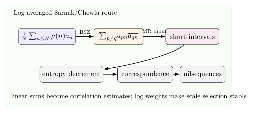
这篇笔记想整理的是 Sarnak 猜想的一条现代路线:从莫比乌斯函数和零熵动力系统的正交性出发,经过 Bourgain-Sarnak-Ziegler 准则,把线性相关和转成双线性相关;再借助 Matomaki-Radziwill 的短区间乘法函数估计,以及 Tao 的 entropy decrement,把问题推向对数平均 Chowla 猜想。
1. Sarnak 猜想的基本形状
Sarnak 猜想说,如果 $(X,T)$ 是零拓扑熵动力系统,$f\in C(X)$,那么对任意 $x\in X$,莫比乌斯函数与观测序列 $f(T^n x)$ 应该正交:
$$\frac1N\sum_{n\le N}\mu(n)f(T^n x)\to 0.$$
这里的哲学是:$\mu(n)$ 携带素数分布中的振荡,而零熵系统产生的是低复杂度的确定序列;二者不应该长期对齐。
最简单的有限动力系统情形已经包含素数定理和算术级数中的素数定理。圆周无理旋转情形则接近 Davenport 型估计:对任意无理数 $\alpha$,指数序列 $e(n\alpha)$ 与 $\mu(n)$ 的相关和具有消失。
2. 从 Sarnak 到 Chowla
Chowla 猜想更像是对 $\mu$ 或 Liouville 函数自身随机性的表述。一个典型的 $k$ 点相关形式是
$$\frac1N\sum_{n\le N}\lambda(n+h_1)\cdots \lambda(n+h_k)\to 0,$$
其中 $h_i$ 两两不同。Sarnak 关心的是乘法函数与低复杂度确定序列的相关,Chowla 关心的是乘法函数自身不同平移之间的相关。二者之间可以用 Furstenberg correspondence principle 和动力系统模型联系起来。
对数平均版本把普通平均换成
$$\frac1{\log N}\sum_{n\le N}\frac{a(n)}n.$$
这个权重让尺度选择更加稳定,也更适合短区间分析。很多情况下,对数平均结论比普通平均结论先被证明,因为它容许把不同尺度上的误差以更柔和的方式叠加。
3. Bourgain-Sarnak-Ziegler 准则
BSZ 准则的核心是一个线性到双线性的转换。设 $a_n$ 是有界序列,如果对很多不同素数 $p\ne q$,都有
$$\frac1N\sum_{n\le N}a_{pn}\overline{a_{qn}}\to 0,$$
那么可以推出
$$\frac1N\sum_{n\le N}\mu(n)a_n\to 0.$$
直观上,$\mu$ 的乘法结构允许我们把原来的线性相关拆成不同素数伸缩后的相关。对角部分 $p=q$ 用平凡估计和体积小来处理;非对角部分则由上面的假设控制。这一点和 Calderon-Zygmund 分解的精神很像:把难对象拆成一个小的对角坏集和一个可估计的非对角主体。
4. Matomaki-Radziwill 的短区间输入
Matomaki-Radziwill 的工作说明,乘法函数在大多数短区间里的平均行为可以被控制。粗略地说,对许多短区间 $[x,x+H]$,有
$$\frac1H\sum_{x 接近它在长区间中的平均。这使得我们可以把一个全局相关和切成许多短尺度,再用欧拉乘积、二阶矩和组合恒等式逐层比较。 短区间估计真正有用的地方在于:它让乘法函数的局部随机性可以被拿来攻击动力系统中的相关问题,而不是只停留在平均阶的数论命题。 entropy decrement 的思想是寻找一个尺度,使得随机变量 $n$ 与它的素数倍 $pn$ 之间的条件信息变少。换句话说,在合适尺度上,系统看到的结构不会因为乘一个小素数而增加太多复杂度。 这一步的意义是把“乘法平移”转成“动力系统里可比较的两个观测”。当这个信息损失足够小的时候,短区间估计、BSZ 双线性结构和 correspondence principle 就可以接上。 nilsequence 是零熵系统中非常重要的一类模型。它既有足够丰富的几何结构,又保留了可计算的 Fourier 分析。把 Sarnak、Chowla、短区间乘法函数和 nilsequence 放在一起看,真正的问题是:乘法函数的随机性如何穿过 nilmanifold 上的低复杂度轨道。 这条路线目前最有价值的地方,不是把所有情形一次性解决,而是提供了一张方法地图:线性相关转双线性相关;短区间估计提供局部随机性;entropy decrement 选择尺度;Furstenberg 原理把数论相关放回动力系统。5. Entropy decrement 的作用
6. Nilsystem 方向