Symplectic geometry – github-backend

旧博客原文

原题：Symplectic geometry

1. Introduction

This is the first note of a series of notes concert on semiclassical analysis. Given the basic material on symplectic geometry. Including the following material,

The case at a point, or we can look it as the case in ${{\mathbb R}^{2n}}$ .
The standard material in symplectic geometry, i.e. Hamiltonian mechanics, two approach, global one concentrating on lie derivative, and a locally one concentrating on the power of Darboux theorem, i.e. the existence of a canonical coordinate.
The basic facts on Poission bracket.
The basic facts on Lagrange sub-manifold, and the involve of Liouville measure.

2. Case of a point, or ${{\mathbb R}^{2n}}$

Let ${V: {\mathbb R}^n \rightarrow {\mathbb R}^n}$ be a vector field, at once we have a vector field, we could consider the associated flow of it,

$\displaystyle \left\{ \begin{aligned} \overset{\cdot}\omega & = & V(\omega)\\ \omega(0) & =&z \end{aligned} \right. \ \ \ \ \ (1)$

express the trajectory start from ${z}$ along the vector field.

Remark 1 There ${\overset{\cdot}\omega:=\frac{\partial \omega}{\partial t}}$ . One the other hand, due to the locally existence theorem of ODE, if the regularity of ${V}$ is enough, then the solution exist and is uniqueness.

Definition 1 ${\psi_t z=\omega(t,z)}$ or more convenient ${\psi_t:= exp(tV)}$ . We call ${\{\psi_t\}_{t\in {\mathbb R}}}$ the flow map or the exponential map generated by ${V}$ .

Lemma 2 For flow map, we have following:

${\psi_0z=z}$ for all ${z\in {\mathbb R}^N}$ .

${\psi_{t+s}=\phi_t\psi_s}$ for all ${s,t\in {\mathbb R}}$ .

for each time ${t\in {\mathbb R}}$ , the mapping ${\psi_t: {\mathbb R}^n\rightarrow {\mathbb R}^n}$ is a diffeomorphism with ${(\psi_{t})^{-1}=\psi_{-t}}$

So it is a group action on ${{\mathbb R}^n}$ , with units as diffeomorphism of ${{\mathbb R}^n}$ . Proof:

This lemma is the direct corollary of the theory of ODE. $\Box$

Now let us special to the case ${{\mathbb R}^{2N}={\mathbb R}^n\times {\mathbb R}^n}$ . In local coordinate we have ${z=(x,\xi)}$ , ${x\in {\mathbb R}^n}$ express position of particle, ${\xi \in {\mathbb R}^n}$ express momentum of particle.

Definition 3 ${z=(x,\xi),w=(y,\eta )}$ in ${{\mathbb R}^{2n}}$ define their symplectic product,

$\displaystyle \sigma(z,w):=<\xi,y>-<x,\eta> \ \ \ \ \ (2)$

In a matrix form, ${\sigma}$ coincide with a ${2n\times 2n}$ matrix

$\displaystyle J=\begin{pmatrix} 0 & I \\ -I & 0\end{pmatrix} \ \ \ \ \ (3)$

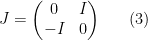
Following lemma given the basic property of ${\sigma, J}$ .

Lemma 4 The following basic property are true.

${\sigma(z,\omega)=<Jz,w>}$ , ${\forall z,w \in {\mathbb R}^{2n}.}$

the bilinear form ${\sigma}$ is antisymmetric, ${\sigma(z,w)=-\sigma(w,z)}$ and degenerate, i.e. if ${\sigma(z,w)=0}$ for all ${w\in {\mathbb R}^{2n}}$ , then ${z=0}$ .

${J^2=-I}$ , ${J^{T}=-J=J^{-1}}$ .

Proof:

trivial calculate get this.
trivial.
${JJ^{-1}=-I}$ , by basic linear algebra everything follows.

$\Box$

3. Hamiltonian mechanics

Definition 5 Symplectic form: non-degenerate closed 2 form in a standard coordinate(Darboux coordinate, coordinate like ${{\mathbb R}^{2n}}$ ) looks like,

$\displaystyle \begin{pmatrix} 0 & -I \\ I & 0 \end{pmatrix} \ \ \ \ \ (4)$

${\forall x\in X}$ , map

$\displaystyle T_xX\rightarrow T_x^*X$

$\displaystyle v\rightarrow w(\cdot, v)$

is an isomorphism. ${w}$ is called the symplectic form.

There is locally coordinate for ${TM,T^*M}$ , i.e.,

$\displaystyle TM:\frac{\partial}{\partial x_1},...,\frac{\partial}{\partial x_n}$

$\displaystyle T^*M:dx_1,...,dx_n$

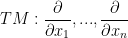
So ${w=f^{ij}dx_i\wedge dx_j}$ , roughly we have ${w(\frac{\partial}{\partial x_k},\frac{\partial}{\partial x_i})=f^{ik}-f^{ki}}$ , this is of course not true, but morally true. Now let us give the definition of symplectic manifold and the relationship of Hamiltonian mechanics.

Definition 6 We have the following definition,

A symplectic manifold is a pair ${(X,\omega)}$ where ${X}$ is a smooth manifold and ${w}$ is a closed two-form on ${X}$ such that ${\forall x\in X}$ the map,
$\displaystyle T_xX\rightarrow T_x^*X$

$\displaystyle v\rightarrow w(\cdot,v)$

is an isomorphism, ${w}$ is called the symplectic form.

If ${(X,w)}$ is symplectic, and ${f:X\rightarrow {\mathbb R}}$ is differentiable, the hamiltonian vector field of ${f}$ is the field ${\Xi_f}$ on ${X}$ whose image under the previous map is ${df}$ . In other word, ${\Xi_f}$ is characticed by the property,
$\displaystyle w(\cdot,\Xi_f)=df(\cdot)$

The flow of ${\Xi_f}$ will be referenced to as the hamiltonian flow of ${f}$ .

Lemma 7 If ${X=R^{2n}}$ coordinate ${(x_1,...,x_n,p_1,...,p_n)=(x,p)}$ and the symplectic form

$\displaystyle w=\sum_{j=1}^ndp_j\wedge dx_j$

then,

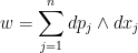
If ${f:{\mathbb R}^{2n}\rightarrow {\mathbb R}}$ is differentiable, then the integral curves of ${\Xi_f}$ are the solutions to the system of ODEs,
$\displaystyle \left\{ \begin{aligned} \overset{\cdot}x_j & = & \frac{\partial f}{\partial p_j}\ \ \ j=1,2,...,n \\ \overset{\cdot}p_j & =& -\frac{\partial f}{\partial x_j} \ \ \ j=1,2,...,n \\ \end{aligned} \right. \ \ \ \ \ (5)$

Moreover, if
$\displaystyle f(x,p)=\frac{1}{2m}\|p\|^2+V(x). \ \ \ \ \ (6)$

Where ${V}$ is a smooth solution (“potential”), and ${(x(t),p(t))}$ is a trajectory of the Hamiltonian flow of ${f}$ , then

$\displaystyle m\overset{\cdot\cdot}x=-\nabla \ \ \ \ \ (7)$

This is the Newton’s second law for the force ${-\nabla V}$ .

Proof: ${w=\sum_{j=1}^n dp_j\wedge dx_j}$ , due to we have ${w(\cdot, \Xi_f=)=df}$ . So ${\forall j}$ we have:

$\displaystyle w(\frac{\partial}{\partial p_j},\Xi_f) = df(\frac{\partial}{\partial p_j})=\frac{\partial f}{\partial p_j} \ \ \ \ \ (8)$

Assume ${\Xi_f=\lambda^i \frac{\partial}{\partial x_i}+\gamma^i\frac{\partial}{\partial p_i}}$ . Then we have,

$\displaystyle \begin{array}{rcl} \frac{\partial f}{\partial p_j} & = & w(\frac{\partial}{\partial p_j},\lambda^i\frac{\partial}{\partial x_i}+ \gamma^i\frac{\partial}{\partial p^i})\\ & = & \lambda^j\cdot (-1)^{\sigma(...)} \end{array}$

and also,

$\displaystyle \begin{array}{rcl} \frac{\partial f}{\partial x_j} & = & w(\frac{\partial}{\partial p_j},\lambda^i\frac{\partial}{\partial x_i}+ \gamma^i\frac{\partial}{\partial p^i})\\ & = & \gamma^j\cdot (-1)^{\sigma(...)} \end{array}$

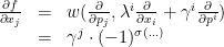
Combine with the definition of integral curve we derive the integral curves of ${\Xi_f}$ i.e. ${\gamma(t)}$ such that ${\overset{\cdot}\gamma(t)=\Xi_f}$ , ${\gamma(t)=(x_1(t),...,p_n(t))}$ is given by 5.

Now we begin to proof the Newton second law for the force ${-\nabla V}$ . We consider the 2-dimensional case at first. We have,

$\displaystyle \begin{array}{rcl} m\overset{\cdot\cdot}x & = & m(\overset{\cdot} {\frac{\partial f}{\partial p}})\\ & = & m\frac{\partial}{\partial t}(\frac{\partial f}{\partial p})\\ & = & m\frac{\partial}{\partial p}[\frac{\partial}{\partial t}(\frac{\|p\|^2}{m}+V(x))]\\ & = & m\frac{\partial }{\partial p}(\frac{2p\overset{\cdot}p}{m}+\frac{\partial V(x)}{\partial x}\cdot \frac{\partial f}{\partial p}) , due\ to \ -\frac{\partial f}{\partial x}=-\frac{\partial V(x)}{\partial x}.\\ & = & m\frac{\partial }{\partial p}(\frac{2p(-\frac{f}{\partial x})}{m}+\frac{\partial V(x)}{\partial x}\cdot \frac{\partial f}{\partial p})\\ & = &-\frac{\partial V(x)}{\partial x} \end{array}$

The high dimension case is similar, thanks to the linearity of ${V}$ and ${\overset{\cdot\cdot}x}$ . $\Box$

Remark 2 Two make Newton’s second law to be true, the form 6 play a crucial role. Is there some generalization of this type of result to more general case, roughly speaking, it is reasonable to expect this could still be true if the hamiltonian function could be divide into potential energy part and kinetic energy part. And the describe of potential energy part is that it is given by a quadratic form.

Lemma 8 In general, for any Hamilton field ${\Xi_f}$ one has:

${\pounds_{\Xi_f}f=0}$ , conservation of energy. In orther word, ${\Xi_f}$ is everywhere tangent to the level sets of ${f}$ .

${\pounds_{\Xi_f}\omega=0}$ , so the Hamiltonian flow of ${f}$ consists of automorphism of ${M,\omega}$ .

General speaking, to proof a theorem on manifold, there always have two choice, coordinate free proof and proof in a careful choose coordinate. If we choose to believe the Darboux theorem 9 is true, the meaning of it is that locally the symplectic manifold are the same.

Proof: If we believe the Darboux theorem 9 is true. then consider in a standard coordinate ${(x_1,...,x_n,p_1,...,p_n)}$ , we have,

$\displaystyle \Xi_f=\sum_{i}\frac{\partial f}{\partial x_i}\frac{\partial}{\partial p_i}-\sum_{i}\frac{\partial f}{\partial p_i}\frac{\partial}{\partial x_i} \ \ \ \ \ (9)$

So of course ${\pounds_{\Xi_f}f=\Xi f=0}$ . In general case, i.e. coordinate free proof, ${\omega(\cdot,\Xi_f)=df}$ . Use identity if lie derivative. The second thing is also easy to proof by look in a local canonical coordinate, involve the indentity of lie derivative. $\Box$

Remark 3 I need more understanding on the lie derivative, see wiki.

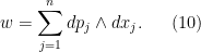
Theorem 9 (Darboux theorem) Near any point there exist coordinate: ${(x_1,...,x_n,p_1,...,p_n)}$ usually called Darboux coordinates, such that the sympletic form ${w}$ has the form,

$\displaystyle w=\sum_{j=1}^ndp_j \wedge dx_j. \ \ \ \ \ (10)$

Remark 4 This theorem means there do not exist local invariant in symplectic manifold.

Proof: $\Box$

\newpage

Theorem 10 If ${M}$ is any smooth manifold, then its cotangent bundle ${X=T^*M}$ has a natural symplectic structure.

Proof: we have local coordinate on ${T^M}$ derive from ${(x_1,...,x_n,dx_1,...,dx_n)}$ , it is ${(x_1,...,x_n,p_1,...,p_n)}$ . Remember we have Riemann metric: ${g^{ij}dx_idx_j}$ on ${T^*M\otimes T^*M}$ , the existence of Riemann metric involve a unit decomposition argument and bump function, I just recall it there. Now we move on, consider the relationship between ${M,TM,T^*M}$ .

$\displaystyle M{\longleftrightarrow} T^*M\overset{pairing, (X,f)=X(f)} {\longleftrightarrow} TM \ \ \ \ \ (11)$

$\Box$

Remark 5 It need not be the case that ${\alpha}$ non-degenerate ${\Longrightarrow}$ ${d\alpha}$ non-degenerate. This case in the lemma is a example to show that could be the case: ${\alpha}$ degenerate ${\Longrightarrow}$ ${d\alpha}$ non-degenerate. We glue something together on the space pf differential operator to understand the topology of it but not deifferential structure or more refinement structure. Quntalization could be look as a way to glue, this could be down if there is a differential equation with some special condition (come from a flow take charge of it suffice).

Lemma 11 (The proof of ${d\alpha}$ is non-degenerate) Let ${(x_1,...,x_n)}$ be local coordinates on ${U\subset M}$ . Define a coordinate system ${(x_1,...,x_n,p_1,...,p_n)}$ on ${T^*U}$ by the condition:

$\displaystyle \forall \xi\in T^*_{x}U, p_j(\xi)=\xi(\frac{\partial}{\partial x_j}) \ \ \ \ \ (12)$

Prove that in Darboux coordinate, ${\alpha=\sum_{j=1}^n p_jdx_j}$ and therefore ${\omega=\sum_{j=1}^n dp_j\wedge dx_j}$ .

Proof: $\Box$

Theorem 12 Let ${(M,g)}$ be a smooth Riemann manifold and let ${f:T^*M\rightarrow {\mathbb R}}$ be one half of the square of the Riemann norm, so that in local coordinate,

$\displaystyle f(x,p)=\frac{1}{2}\sum_{i,j}g^{ij}p_ip_j \ \ \ \ \ (13)$

Then the trajectorics of the hamiltonian flow of ${f}$ , projected down to ${M}$ , are geodesic aries in this fashion.

Newton’s second law+ energy vanish.

Proof:

$\displaystyle m\overset{\cdot\cdot}x=\nabla V=0$

So second variation formula describe of geodesic give us the fact that the trajective is geodesic. $\Box$

Remark 6 We could directly calculate in local coordinate.

4. Poisson brackets

${f}$ is the Hamiltonian generating the dynamic ${g}$ is any smooth function on phase space (the symplectic manifold), then the rate of change of ${g}$ along the trajectraries of d is the function

$\displaystyle \overset{\cdot}g=\pounds_{\Xi_f}g=d_g(\Xi_f)=\omega(\Xi_f,\Xi_g) \ \ \ \ \ (14)$

Definition 13 If ${(X,\omega)}$ is symplectic and ${f,g\in C^{\infty}(X)}$ , the poisson bracket of ${f}$ and ${g}$ is defined to be the function on ${X}$ .

$\displaystyle \{f,g\}:=\omega(\Xi_f,\Xi_g) \ \ \ \ \ (15)$

Lemma 14 In canonical (Darboux) coordinate where ${\omega=\sum_j dp_j\wedge dx_j}$ , one has,

$\displaystyle \{f,g\}=\sum_{j=1}^n\frac{\partial f}{\partial p_j}\frac{\partial g}{\partial x_j}-\frac{\partial f}{\partial x_j}\frac{\partial g}{\partial p_j} \ \ \ \ \ (16)$

In particular, ${\{p_j,x_j\}=\delta_{ij}}$ .

Proof:

$\displaystyle \begin{array}{rcl} \{f,g\} & = & \omega(\Xi_f,\Xi_g)\\ & = & \sum_{j=1}^n dp_j\wedge dx_j(-\frac{\partial f}{\partial p_j}\frac{\partial}{\partial x_j}+\frac{\partial f}{\partial x_j}\frac{\partial}{\partial p_j}, -\frac{\partial g}{\partial p_j}\frac{\partial}{\partial x_j}+\frac{\partial g}{\partial x_j}\frac{\partial}{\partial p_j} )\\ & = & \sum_{j=1}^n\frac{\partial f}{\partial p_j}\frac{\partial g}{\partial x_j}-\frac{\partial f}{\partial x_j}\frac{\partial g}{\partial p_j}. \end{array}$

$\Box$

Theorem 15 If ${(X,\omega)}$ is a symplectic manifold then ${\{C^{\infty}(X),\{\cdot\}\}}$ is a Lie algebra.

Proof: Bilinearty, skew-symmetric come form,

$\displaystyle \{f,g\}=\omega(\Xi_f,\Xi_g) \ \ \ \ \ (17)$

Jacobi identity:

$\displaystyle \{\{f,g\},h\}+\{\{g,h\},f\}+\{\{h,f\},g\}=0 \ \ \ \ \ (18)$

could be proved by calculate under a local coordinate. $\Box$

补充说明

以下是新整理的中文说明；上方旧博客原文保持不变。

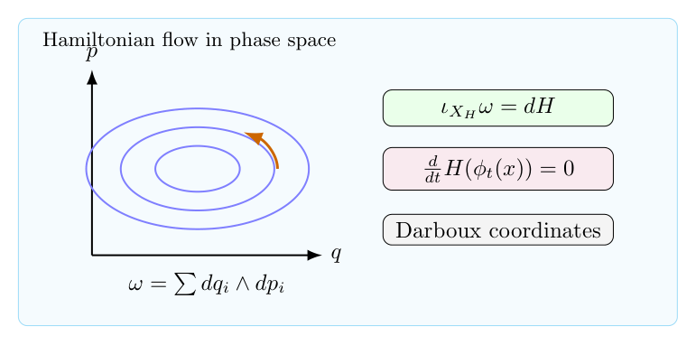
辛几何是半经典分析和 Hamiltonian mechanics 的共同语言。它研究的不是长度和角度，而是相空间中的面积形式、Hamiltonian flow 以及由此产生的守恒结构。这篇笔记从向量场的 flow 开始，逐步进入 symplectic form、Darboux theorem 和 Poisson bracket。

辛几何笔记：Hamiltonian flow、Darboux 坐标与 Poisson bracket — Hamiltonian flow 在相空间中沿能量面运动，并保持 symplectic form。

1. 从向量场到 flow

给定光滑向量场 $V$，它生成常微分方程

$$\frac{d}{dt}\phi_t(x)=V(\phi_t(x)),\qquad \phi_0(x)=x.$$

若解存在且唯一，那么 $\phi_t$ 满足群性质

$$\phi_{t+s}=\phi_t\circ \phi_s,\qquad \phi_0=\operatorname{id}.$$

因此一个向量场不仅给出每个点的速度，也给出整个空间上的一参数 diffeomorphism group。

2. 标准相空间

在 Hamiltonian mechanics 中，标准相空间是 $\mathbb R^{2n}$，坐标写成

$$(q_1,\ldots,q_n,p_1,\ldots,p_n),$$

其中 $q$ 是位置，$p$ 是动量。标准 symplectic form 是

$$\omega=\sum_{j=1}^n dq_j\wedge dp_j.$$

它是闭的、非退化的二形式。非退化性意味着每个一形式都可以唯一对应一个向量场。

3. Hamiltonian vector field

给定能量函数 $H$，Hamiltonian vector field $X_H$ 由

$$\iota_{X_H}\omega=dH$$

定义。在标准坐标下，这给出 Hamilton 方程

$$\dot q_j=\frac{\partial H}{\partial p_j},\qquad
\dot p_j=-\frac{\partial H}{\partial q_j}.$$

若 $H(q,p)=\frac12|p|^2+V(q)$，那么 Hamilton 方程化成 Newton 方程

$$\ddot q=-\nabla V(q).$$

所以经典力学可以看成辛几何中的一条 flow。

4. 守恒与 Darboux theorem

Hamiltonian flow 保持能量：

$$\frac{d}{dt}H(\phi_t(x))=dH(X_H)=\omega(X_H,X_H)=0.$$

它也保持 symplectic form，即 $\phi_t^\ast\omega=\omega$。这比保持体积更强，是 Hamiltonian 系统的基本刚性。

Darboux theorem 说，任意 symplectic manifold 在局部都可以选坐标，使得

$$\omega=\sum dq_j\wedge dp_j.$$

这说明辛流形没有类似曲率那样的局部不变量；它的困难主要来自全局拓扑和 Lagrangian 子流形的相互位置。

5. Poisson bracket

两个函数 $f,g$ 的 Poisson bracket 定义为

$$\{f,g\}=\omega(X_f,X_g).$$

在标准坐标下，

$$\{f,g\}=\sum_j\left(\frac{\partial f}{\partial q_j}\frac{\partial g}{\partial p_j}
-\frac{\partial f}{\partial p_j}\frac{\partial g}{\partial q_j}\right).$$

沿 Hamiltonian flow 的演化满足

$$\frac{d}{dt}f(\phi_t(x))=\{f,H\}(\phi_t(x)).$$

这就是从几何到动力系统、再到半经典分析的接口：量子力学里的 commutator 在半经典极限中对应 Poisson bracket。

分类： Symplectic geometry

辛几何笔记：Hamiltonian flow、Darboux 坐标与 Poisson bracket

旧博客原文

补充说明

1. 从向量场到 flow

2. 标准相空间

3. Hamiltonian vector field

4. 守恒与 Darboux theorem

5. Poisson bracket