不确定性原理：局部化、Bernstein 估计与 Gaussian

旧博客原文

原题：Uncertainty principle

The pdf version is Uncertainty principle. The nice note of terrence tao seems given a nice answer for the problem below.

1. Introduction

Is there a Brunn-Minkowski inequality approach to the phenomenon charged by uncertainty principle? More precisely, is it possible to say some thing about the Gaussian distribution

$\displaystyle G(x)=e^{-|x|^2} \ \ \ \ \ (1)$

to be the best choice that ${\|\hat G-G\|_2}$ arrive minimum?

Remark 1 Or some other suitable distance space on reasonable function (may be some gromov hausdorff distance? Any way, to say the guassian distribution is the best function to defect the influence of uncertain principle.

I do not know the answer of the problem 1, but this is a phenomenon of a universal phylosphy, aid, uncertainty principle, heuristic:

It is not possible for both function ${f}$ and its Foriour transform ${\hat f}$ to be localized on small set.

Now let me give some approach by intuition to explain why the phenomenon of “uncertainty principle” could happen.

The approach is based on:

level set decomposition.
area formula (or coarea formula), anyway, some kind of change variable formula.
integral by part.
Basic understanding on exponential sum.

Let our function ${f\in S}$ the Shwarz space, we begin with a intuition (not very rigorous) calculate:

$\displaystyle \begin{array}{rcl} \hat f(\xi) & = & \int e^{2\pi i<\xi, x>}f(x)dx\\ & \overset{integral \ by \ part}= &\int \frac{1}{-2\pi i\xi}e^{-2\pi i<x,\xi>}\cdot \nabla f(x)\\ & \overset{Fubini}= & \int_{inf |f|}^{max |f|}\int_{level set A(t)} \frac{-e^{2\pi i<\xi,x>}}{-2\pi i\xi}\nabla f(x)dH^{n-1}(A)dt \end{array}$

Now we try to understanding the result of the calculate, it is,

$\displaystyle \hat f(\xi) =\int_{inf |f|}^{max |f|}\int_{level set A(t)} \frac{-e^{2\pi i<\xi,x>}}{-2\pi i\xi}\nabla f(x)dH^{n-1}(A)dt \ \ \ \ \ (2)$

$\displaystyle \pounds(A(t),\xi)=\int_{level set A(t)} \frac{-e^{2\pi i<\xi,x>}}{-2\pi i\xi}\nabla f(x)dH^{n-1}(A) \ \ \ \ \ (3)$

The calculate is wrong, but not very far from the thing that is true, the key point is now the exponential sum involve. We could use the pole coordinate in the frequence space and get some very rough intuition of why the the uncertainty principle could occur.

Remark 2 Why we consider the level set decomposition, due to the integral is a combination of linear sum of the integral on every level set, so shape of level set is the key point.

The part of ${\frac{-e^{2\pi i<\xi,x>}}{-2\pi i\xi}}$ in 2 is a rotation on the level set, a wave correlation of it and the christization function ${\chi_{A_t}}$ of level set ${A_t}$ in the whole space, this is of course a exponential sum.

Now we can begin the final intuition explain of the phenomenon of uncertainty principle. If the density of function ${f}$ is very focus on some small part of the physics space, then it is the case for level sets of ${f}$ , but we could say some thing for the exponential sum ${\pounds(A(t),\xi)}$ 3 related to the level set, just by very simply argument with hardy litterwood circle method or Persaval identity? Any way, something similar to this argument will make sense, due to if the diameter of level set focus ois small, then we can not get a decay estimate for ${\pounds(A(t),\xi)}$ when ${\xi\rightarrow \infty}$ along one direction in frequency space, in fact we could say the inverse, i.e. it could not decay very fast.

2. Bernstein’s bound and Heisenberg uncertainty principle

2.1. Motivation and Bernstein’s bound

There is two different Bernstein’s bound, we discuss the first with the motivation, and proof the second rigorously. \paragraph{Form 1} ${A}$ is a invertible affine map, then for a ball ${B}$ , ${A(B)=\epsilon}$ is a ellipsoid.

$\displaystyle \epsilon=\{x\in {\mathbb R}^d|\sum_{j=1}^{d}r_j^{-2}(x_j-y_j)^2\leq 1\} \ \ \ \ \ (4)$

By a orthogonal transform we could make ${A}$ to be a diagonal matrix, i.e. ${A=diag(r_1,...,r_d)}$ . It is said, for ${\forall f\in S}$ or ${f}$ is a smooth bump function, ${f_A=f\circ A^{-1}}$ , so we have,

$\displaystyle \hat f_A(\xi)=\int e^{2\pi i<x,\xi>}\cdot f\circ A^{-1}(x)dx \ \ \ \ \ (5)$

We define dual of ${\epsilon}$ , ${\epsilon^*:=\{\xi\in {\mathbb R}^d| \sum_{j=1}^d\xi_j^2r_j^2\leq 1\}}$ .

Remark 3 Why there we use the metric ${\xi_j^2r_j^2\leq 1}$ but not the standard inner product ${<\xi,x>}$ ? How to understand the choice?

Proposition 1 We have the following property:

${f_A\in L^{\infty}\Longrightarrow \|\hat f_A\|_{1}\leq +\infty}$ .

${|\hat f_A(\xi)|\leq c_N|\xi|(1+|\xi|^2_{\epsilon^*})^{-N}}$

Remark 4

$\displaystyle |\xi|^2_{\epsilon^*}=\sum_{i=1}^d\xi_j^2r_j^2$

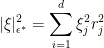
This is a norm of ${{\mathbb R}^d}$ related to ${\epsilon^*}$ .

Proof: Suffice to proof 2.

$\displaystyle \begin{array}{rcl} |\hat f_A(\xi)| & = & |\int_{{\mathbb R}^d}e^{2\pi i<x,\xi>}f_A(x)dx|\\ & \overset{integral \ by \ part}\sim & \frac{1}{(1+|\xi|)^N}\int |e^{2\pi i<x,\xi>}\partial^N f_A(x)dx|\\ & = & c_N |\xi|(1+|\xi|_{\epsilon^*}^2)^{-N} \end{array}$

$\Box$

More quantitative we have rigorous one: \paragraph{Form 2} If ${f\in L^2({\mathbb R}^d)}$ , ${supp f\in B(r,0)}$ , then it is not possible for ${\hat f}$ to be concentrate on a scale much less than ${R^{-1}}$ .

Proposition 2 (Bernstein’s bound) Suppose ${f\in L^2({\mathbb R}^d)}$ , ${supp f\subset B_R(0)}$ . Then,

$\displaystyle \|\partial^{\alpha}\hat f\|_2\leq (2\pi r)^{|\alpha|}\|f\|_2, \forall \alpha. \ \ \ \ \ (6)$

Proof: ${\alpha=0}$ case is trivial by Paserval identity, which said on ${L^2({\mathbb R}^d)}$ , fourier transform is a isometry, ${\|f\|_2=\|\hat f\|_2}$ . For general case, integral by part, and use trivial estimate,

$\displaystyle \begin{array}{rcl} \|\partial^{\alpha}\hat f\|_2 & \overset{integral \ by \ part}= & \|x^{\alpha} f\|_2\\ & \leq & (2\pi r)^{\alpha}\|f\|_2 \end{array}$

$\Box$

2.2. Heisenberg inequality

Theorem 3 (Heisenberg uncertain principle) ${f\in L^2({\mathbb R}^d)}$ , so ${\hat f\in L^2({\mathbb R}^d)}$ , ${\|f\|_2=\|\hat f\|_2}$ . then for any ${x_0,\xi_0\in {\mathbb R}^d}$ , every direction, we have

$\displaystyle \|f\|_2^2=\|f\|_2\|\hat f\|_2\leq \|(x-x_0)f\|_2\|(\xi-\xi_0)\hat f\|_2 \ \ \ \ \ (7)$

Remark 5 We could understand the inequality by the following way. suffice to prove it with ${f\in S}$ and then by approximation argument. ${f\otimes \hat f\in S({\mathbb R}^d\times {\mathbb R}^d)}$ , define ${\|f\otimes \hat f\|_2:= \|f\|_{L^2({\mathbb R}^d)}\cdot \|\hat f\|_{L^2({\mathbb R}^d)}}$ . then we have the following:

$\displaystyle \|f\otimes \hat f\|_{L^2}\leq 4\pi \|xf\otimes \hat{xf}\|_{L^2} \ \ \ \ \ (8)$

Remark 6 The inequality is shape, the extremizers being precisely given by the modulated Gaussians: arbitrary

$\displaystyle f(x)= c e^{2\pi i\xi_0x}e^{-\pi \delta(x-x_0)^2} \ \ \ \ \ (9)$

There are two proof strategies I have tried, I try them for several hour but not work out with a satisfied answer, the method more involve, I explain what happen in section 1, I have not tried, I will try it later. Both this two strategies i face some difficulties, I explain why I can not work out them with a proof: \paragraph{Strategy 1} The first one is, we could work with ${f\in S}$ of course, by approximation, then we find, by Paserval, ${\|f\|_2=\|\hat f\|_2, \|\partial_x f\|_2=\|\xi \hat f\|2}$ and are both true. then we use our favourite way to use Cauchy-Schwarz, the difficulty is we can not use a integral by part argument directly, even after restrict ourselves with monotonic radical symmetry inequality and by a rearrangement inequality argument, it seems reasonable due to rearrangement decreasing the kinetic energy as said in Lieb’s book. But even work with monotonic one, then one involve with some complicated form, try to use Fubini theorem to rechange the order of integral try to say something, it is possible to work out by this way but I do not know how to do. There is some calculate under this way,

$\displaystyle \begin{array}{rcl} \|xf\|_2\|\xi \hat f\|_2 & \overset{Cauchy-Schwarz}\geq & \int xf\cdot \partial_x f\\ & \sim & \int f^2 \end{array}$

but you know, at a point we have ${\partial_x(Xf)=f+x\partial_x f\neq f}$ , the reasonable calculate is following,

$\displaystyle \partial_x(xf)=f+x\partial_x f \ \ \ \ \ (10)$

We want ${\partial_x P(x,f) =f}$ , Then

$\displaystyle \begin{array}{rcl} \partial_x P(x,f) & = & f\\ & = & \partial_x(xf)-x\partial_x f\\ & = & \partial_x(xf)-\partial_x(\frac{1}{2}x^2\partial_x f)+\frac{1}{2}x^2\partial_{x^2}f\\ & = & \partial_x(\frac{1}{6}x^3\partial_{x^2}f)-\frac{1}{6}x^3\partial_{x^3}f\\ ...\\ & = &\partial_x(\sum_{i=1}^{\infty}(-1)^{i+1}x^i\frac{1}{i!}\partial_{x^i}f)+(-1)^{i+1}x^i\frac{1}{i!}\partial_{x^{i+1}}f \end{array}$

Seems to be ${f=\partial_x(ln(f))}$ … I do not know.

\paragraph{Strategy 2} The second strategy is, in the quantity ${\|xf\|_2\|\xi \hat f\|_x}$ we lose two cone very near ${x_0,\xi}$ , we need use the extra thing to make up them. May be effective argument come from some geometric inequality.

3. The Amerein-Berthier theorem

Next we investigate following problem, the problem is following: if ${E,F\subset {\mathbb R}^d}$ are of finite measure, can there be a nonzero ${f\in L^2({\mathbb R}^d)}$ with ${supp (f)\subset E}$ and ${supp(\hat f)\subset F}$ ? Some argument is folowing: Observe that:

$\displaystyle \chi_{F}\hat f=\hat f \Longrightarrow \chi_{E}(\chi_F \hat f)^{\vee}=f. \ \ \ \ \ (11)$

Assume that: ${Tf:=\chi_{E}(\chi_F \hat f)^{\vee}}$ then ${Tf=f}$ . So we have, at least ${\|T\|_{2-2}\geq 1}$ . Some dirty calculate show:

$\displaystyle \begin{array}{rcl} (Tf)(x) & = & \int e^{2\pi i\xi x}\chi_F\hat f(\xi)\chi_E(x)d\xi\\ & = & \int \int e^{2\pi i\xi(x-y)}f(y)\chi_F(\xi)\chi_E(x)dy d\xi\\ & \overset{Fubini}= &\int_{{\mathbb R}^d}\chi_E(x)\chi_F^{\vee}(x-y)f(y)fy \end{array}$

So we can define kernel of ${T}$ ,

$\displaystyle K(x,y)=\chi_E(x)\chi_F(x-y)^{\vee} \ \ \ \ \ (12)$

By Fubini, we calculate the Hilbert-Schmidt norm:

$\displaystyle \int_{{\mathbb R}^{2d}}|K(x,y)|^2dxdy=|E||F|=\sigma^2<+\infty \ \ \ \ \ (13)$

So ${T}$ is a compact operator and its ${L^2}$ operator norm satisfied ${\|T\|=\min(\sigma,1)}$ . So if ${\sigma<1}$ then we can canculate we can not have ${f\neq 0}$ in the original question.

The story is in fact more interesting, the answer of the question is no even for ${\sigma\geq 1}$ , so in all case. We have the following quatitative theorem:

Theorem 4 ${E,F}$ finite measure in ${{\mathbb R}^d}$ , then

$\displaystyle \|f\|_{L^2({\mathbb R}^d)}\leq c(\|f\|_{L^2(E^c)}+\|\hat f\|_{L^2(F^c)}) \ \ \ \ \ (14)$

for some constant ${c=c(E,F,d)}$ .

Remark 7 There is a naive approach for this theorem: Area formula trick, the shape of level set. Obvioudly we have:

$\displaystyle \|f\|_{L^2({\mathbb R}^d)}\leq \|f\|_{L^2(E)}+\|f\|_{L^2(E^c)} \ \ \ \ \ (15)$

Key point is proof:

$\displaystyle \|f\|_{L^2(E)}\leq c(E,F,d)\|\hat f\|_{L^2(F^c)} \ \ \ \ \ (16)$

Let us do some useless further calculate:

$\displaystyle \begin{array}{rcl} |f\|_{L^2(E)} & = & \|\chi_E \cdot f\|_{L^2({\mathbb R}^d)}\\ & = & \|\widehat {\chi_E\cdot f}\|_{L^2({\mathbb R}^d)}\\ & = & \|\hat \chi_E \cdot \hat{f^{\vee}}\|_{L^2({\mathbb R}^d)} \\ & = & \|\chi_E^{\vee} * f^{\vee}\|_{L^2({\mathbb R}^d)} \end{array}$

So suffice to have:

$\displaystyle \|\chi_E^{\vee} * f^{\vee}\|_{L^2({\mathbb R}^d)}\leq c(E,F,d)\|\hat f\|_{L^2(F^c)} \ \ \ \ \ (17)$

But there is connter example given by modified scaling Gaussian distribution… The point is form 15 to 16 is too loose.

Following I given a right approach, following by my sprite on level set and area formula argument and discritization.

Proof: The story is the same for a discretization one. We need point out, change the space ${{\mathbb R}^d}$ to ${{\mathbb Z}^d}$ , then every thing become a discretization one, and the change could been argue as a approximation way. What happen then, we have a naive picture in mind which is:

$\displaystyle \delta \rightarrow wave , \ wave \rightarrow \delta$

What is the case with ${L^2}$ norm, it become the standard nner product on ${{\mathbb Z}^d}$ , and the scale involve, i.e. we have the following basic estimate:

$\displaystyle \|\chi_E f\|_1^2\leq \|\chi_E f\|_2 \cdot|E| \ \ \ \ \ (18)$

Now image if the density of ${f}$ concentrate in a very small area, then by a cut off argument we consider the supp of ${f}$ , ${supp f=E}$ is very small, then use the argument 18, we could conclute the density of ${\hat f}$ could not very concentrate in the fraquence space. The constant ${c(E,F,d)}$ could be given presicely by this way, but I do not care about it. $\Box$

4. Logvinenko-Sereda theorem

Next we formulate some result that provide further evidence of the non-concentration property of functions with Fourier support on ${B_1}$ .

4.1. A toy model

Theorem 5 Let ${\alpha>1}$ an suppose that ${S\subset {\mathbb R}^d}$ satisfies,

$\displaystyle |S\cap B|<\alpha |B|, \ for \ all \ balls \ B \ of \ radius\ 1. \ \ \ \ \ (19)$

If ${f\in L^2({\mathbb R}^d)}$ satisfies ${supp(\hat f)\subset B(0,1)}$ then

$\displaystyle \|f\|_{L^2(S)}\leq \delta(\alpha)\|f\|_2 \ \ \ \ \ (20)$

Where ${\delta(\alpha)\rightarrow 0}$ as ${\alpha \rightarrow 0}$ .

Proof: This is a easy corollary of the argument I give in the proof of Amerein-Berthier theorem 4. $\Box$

4.2. A refine version

Theorem 6 Suppose that a measurable set ${E\subset {\mathbb R}^d}$ satisfies the following “thinkness” condition: there exists ${\gamma\in (0,1)}$ such that

$\displaystyle |E\cap B|>\gamma |B| \ for \ all \ balls \ B \ of \ radius\ R^{-1}. \ \ \ \ \ (21)$

where ${R>0}$ is arbitrary but fixed. Assume that ${supp(\hat f)\subset B(0,R)}$ . Then

$\displaystyle \|f\|_{L^2({\mathbb R}^d)}\leq C\|f\|_{L^2(E)}. \ \ \ \ \ (22)$

where the constant ${C}$ depends only on ${d}$ and ${\gamma}$ .

Remark 8 This proof need some very good estimate come from several complex variables.

5. The Malgrange-Ehrenpreis theorem

Theorem 7 Let ${\Omega}$ be a bounded domain in ${{\mathbb R}^d}$ and let ${p\neq 0}$ be a polynomial, Then, for all ${g\in L^3(\Omega)}$ , there exists ${f\in L^2(\Omega)}$ such that ${p(D)f=g}$ in a distribution sence.

补充说明

以下是新整理的中文说明；上方旧博客原文保持不变。

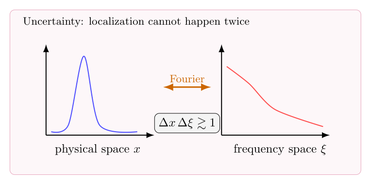
不确定性原理的核心直觉是：一个函数和它的 Fourier transform 不可能同时高度集中。这里的“集中”可以有许多精确版本：支撑大小、方差、指数衰减、带限函数的空间尺度，或者通过 level sets 来衡量的几何集中。

不确定性原理：局部化、Bernstein 估计与 Gaussian — 不确定性原理的基本图像：物理空间中的强集中会迫使频率空间展开，反之亦然。

1. 基本直觉

Fourier transform 把函数分解成平面波：

$$\widehat f(\xi)=\int_{\mathbb R^n}f(x)e^{-2\pi i x\cdot \xi}\,dx.$$

如果 $f$ 集中在很小的物理区域里，那么积分里的相位 $x\cdot \xi$ 在许多方向上变化不够快，$\widehat f$ 就不可能在频率空间里迅速衰减。反过来，如果 $\widehat f$ 被限制在很小的频率球内，$f$ 就必须在物理空间里足够平滑、足够展开。

从 level set 的角度看，$f$ 的每一层都贡献一个振荡积分。level set 的几何形状越小、越刚性，相位平均带来的抵消就越弱。

2. Bernstein 估计

一个非常实用的形式是 Bernstein inequality。若 $\widehat f$ 支撑在半径 $R$ 的球内，那么

$$\|\nabla f\|_{L^p}\lesssim R\|f\|_{L^p}.$$

这说明带限函数不能在尺度远小于 $R^{-1}$ 的区域内剧烈变化。频率支撑越小，物理空间越平滑；频率支撑越大，函数才有能力产生更细尺度的振荡。

更一般地，如果频率支撑在一个椭球中，那么物理空间的自然尺度由对偶椭球控制。这个“对偶尺度”正是不确定性原理的几何版本。

3. Heisenberg 不等式

最经典的方差形式是

$$\left(\int_{\mathbb R^n}|x|^2|f(x)|^2\,dx\right)
\left(\int_{\mathbb R^n}|\xi|^2|\widehat f(\xi)|^2\,d\xi\right)
\ge C_n\|f\|_2^4.$$

一维情形可以通过分部积分和 Cauchy-Schwarz 证明。核心计算是把 $\|f\|_2^2$ 写成 $-\int x\partial_x(|f|^2)$ 的形式，再把 $x f$ 和 $\partial_x f$ 配对。Plancherel 把 $\partial_x f$ 转成频率侧的 $\xi\widehat f$。

4. Gaussian 为什么是极值

Gaussian 同时在物理空间和频率空间保持 Gaussian 形状：

$$f(x)=e^{-\pi |x|^2},\qquad \widehat f(\xi)=e^{-\pi |\xi|^2}.$$

它正好平衡了两个方向的集中，因此在 Heisenberg 型不等式中给出等号情形。这个现象提示一个更几何的问题：是否可以用类似 Brunn-Minkowski 或 entropy convexity 的语言解释 Gaussian 的最优性？

从现代观点看，答案常常与热流、log-Sobolev 不等式和最优输运有关。热流让任意函数逐渐 Gaussian 化；entropy 的凸性则记录了这个过程中的不确定性增加。

5. 一个可继续追问的问题

如果把“集中程度”换成某种几何距离，例如 level sets 的体积增长、分布之间的 transport distance，或者函数图像诱导的度量结构，那么 Gaussian 是否仍然是最自然的最优对象？这个问题不一定有唯一答案，但它把 Fourier 分析里的不确定性和凸几何、概率、几何测度论连在了一起。

不确定性原理：局部化、Bernstein 估计与 Gaussian

旧博客原文

1. Introduction

2. Bernstein’s bound and Heisenberg uncertainty principle

3. The Amerein-Berthier theorem

4. Logvinenko-Sereda theorem

5. The Malgrange-Ehrenpreis theorem

补充说明

1. 基本直觉

2. Bernstein 估计

3. Heisenberg 不等式

4. Gaussian 为什么是极值

5. 一个可继续追问的问题

评论

发表回复 取消回复

更多文章

从支撑接触到 Hausdorff 分层：凸 k-Hessian 解的四步证明机制

From Sum-Free Sets to Strongly 2-Primitive Sets: Localization, Patching, and the Search for Stability

[后端同步测试] 富媒体、代码与数学公式渲染

1

发表回复取消回复