Brunn-Minkowski 不等式：集合加法、离散化与几何 PDE 的影子

旧博客原文

原题：Brunn-Minkowski inequality

In this short note, I posed a conjecture on Brunn-Minkwoski inequality and explain why we could be interested in this inequality, what is it meaning for further developing of some fully nonlinear elliptic equation come from geometry. The main part of the note devoted to discuss several different proof of classical Brunn-Minkowski inequality.

Brunn-Minkowski inequality

1. Introduction

I believe, every type of Brunn-Minkowski inequality, type of Brunn-Minkowski inequality is in some special sense and will be explained later, will be crucial with a corresponding regularity result of a fully nonlinear elliptic equation which could be realizable by geometric way which will also explained in further note.

So the key point is that Brunn-Minkowski inequality is crucial and have potential application, I posed a problem there and then consider the classical Brunn-Minkowski inequality, we give several proof of the classical Brunn-Minkowski inequality, everyone could help us to have a more refine understanding of the original difficulty with different angle.

Theorem 1 (conjecture) We have a map

$\displaystyle f:{\mathbb R}^d\times {\mathbb R}^d \longrightarrow {\mathbb R}^d \ \ \ \ \ (1)$

$\displaystyle (x,y) \longrightarrow f(x,y)$

We are willing to called the function ${f}$ as the hamiltonian function. then we could consider the hamiltonian flow of the function ${f}$ , but this could only true for a even dimension manifold to make there exists ${f}$ that ${df}$ is a non-degenerate closed ${2-}$ form.

Anyway we consider the level set of ${f}$ , we get a foliation i.e ${{\mathbb R}^d=\{\amalg_{p\in {\mathbb R}}f^{-1}(p)\}}$ . we consider the gradient flow with ${f}$ , called the gradient flow begin with ${q\in {\mathbb R}}$ as ${\{\phi_q(t)\}_{t\in {\mathbb R}}}$ . And we wish the gradient flow have a addition structure on itself then we could consider what is the Brunn-Minkowski inequality in this setting, the condition is a group structure on the space of level set ${L_f=\{\amalg_{p\in {\mathbb R}}f^{-1}(p)\}}$ , i.e.

$\displaystyle \forall t_1,t_2\in {\mathbb R}, \forall q\in R^d, \phi_{q}(t_1+t_2)=\phi_{q}(t_1)\circ \phi_{q}(t_2) \ \ \ \ \ (2)$

Remark 1 take ${f(x,y)=x+y}$ in 1, this conjecture reduce to the toy model, i.e. classical Brunn-Minkowski inequality.

Remark 2 We could generate the problem to the problem which is charged by several energy function ${f_1,...,f_k}$ , if the induced gradient flow is amenable, then this is somewhat similar with the one dimension case, I wish if we could do something for the single function ${f_1}$ , then we can say something for the several functions involved case.

Remark 3 This could also generate to amenable group action case and quantization of it.

Meaning, the cohomology induce by a hamiltonian system on some special foliation on fiber of geometric bundle. This type of result could help to establish the vanish of the cohomology, the get the existence theory and regularity result for corresponding elliptic nonlinear differential equation. And solve the original problem I consider.

Now we given the statement of Brunn-Minkowski inequality.

Theorem 2 (brunn minkowski inequality) For ${A,B}$ measurale set in ${{\mathbb R}^d}$ . we have following,

$\displaystyle \mu^{\frac{1}{d}}(A+B)\geq \mu^{\frac{1}{d}}\mu(A)+\mu^{\frac{1}{d}}\mu(B) \ \ \ \ \ (3)$

“>

The general spproach of Brunn-Minkwoski inequality is following,

divide the measurable set ${A,B}$ into small cubes.
Shinking trick, transform the set into convex one.

for the first one, we have the following lemma,

Lemma 3 ${\forall 0<\lambda<1}$ , ${\exists \epsilon>0}$ ${A_{\epsilon}}$ measurable set, ${A_{\epsilon}\subset A}$ , ${\mu(A-A_{\epsilon})<\epsilon}$ , and ${A=(A-A_{\epsilon})\amalg \cup_{i\in I}(c_i\cap A_{\epsilon} ) }$ , and

$\displaystyle \frac{\mu(c_i\cap A_{\epsilon})}{\mu(c_i)}>\lambda, \forall i\in I \ \ \ \ \ (4)$

Proof: The proof of the lemma is a easy corollary of the construction of Lesbegue(or Borel) measurable ${\sigma}$ algebra. $\Box$

Remark 4 The existence of the property given in the lemma is not the key point, the key point is ${d(A_{\epsilon},A)\rightarrow 0, as\ \ \epsilon\rightarrow 0}$ .

Has this two simplify in hand, we could give several approach to proof the inequality and these proof carry information more than just a proof, they carry some information with the structure of space ${(\{ 0,1 \}_{{\mathbb R}^d},\mu^{\frac{1}{d}},+)}$ . \newpage

2. A proof with discretization

There is a lots of ways to attack the Brunn-Minkowski inequality, the most natural one is discretization. But unfortunately there is some technique obstacle for proof or even state the discretization version of “Brunn-Minkowski” inequality.

The “boundary” and “area” should not compatible.

$\displaystyle \mu_{d-1}(\partial E)<<\mu_{d}(\mu(E)) \ \ \ \ \ (5)$

And we need use the fact,

$\displaystyle A_{\epsilon}\overset{G-H \ sence}\longrightarrow A \ \ \ \ \ (6)$

Now we just state what we expect it should transform in, because we have a fully understanding with the discretization model, there is a result named Cauchy-Daveport inequality.

Theorem 4 (cauchy-daveport inequality) There are two case, one in ${{\mathbb Z}}$ , one in finite field ${{\mathbb Z}_p}$ .

${{\mathbb Z}}$ case, ${\forall A,B\subset {\mathbb Z}}$ are finite set,we have,
$\displaystyle |A+B|\geq |A|+|B|-1. \ \ \ \ \ (7)$

${{\mathbb Z}_p}$ case, ${\forall A,B\subset {\mathbb Z}}$ are finite set,we have,
$\displaystyle |A+B|\geq \max\{|A|+|B|-1.p\}. \ \ \ \ \ (8)$

Proof: for the ${{\mathbb Z}}$ case, the story is more or less trivial, just do to a observation, if ${A=\{a_i,a_1<a_2<...<a_n\},B=\{b_i,b_1<b_2<...<b_m\}}$ , then

$\displaystyle a_1+b_1<\min\{a_1+b_2+a_2+b_1\}<....<a_n+a_m$

There exists a strictly increasing chain of length at least ${n+m-1}$ .

For the ${{\mathbb Z}_p}$ case, following is a graph to explain what happen, basically we define a operation on tuples, i.e. ${T:(A,B)\rightarrow (T(A),T(B))}$ , and make the additive energy ${E_{A,B}:=|A+B|}$ decreasing. after induction with this transform and the transform from a tuple to the minimum additive energy by translation, the additive energy decreasing and decreasing then arrive the global minimum. But it is easy to conclude in this case one of ${A,B}$ become null set and then the inequality 8 follows. $\Box$

But when we discrete the Brunn-Minkowski inequality, we expect a high dimension generation of the inequality 4. Naively we wish,

Theorem 5 (naive generation of cauchy-daveport inequality) For ${d\in {\mathbb N}}$ , and ${\forall A,B\subset {\mathbb Z}_d}$ are finite sets,

$\displaystyle |A+B|^{\frac{1}{d}}\geq |A|^{\frac{1}{d}}+|B|^{\frac{1}{d}} \ \ \ \ \ (9)$

But this is not the case, there is a counterexample for 5. We could construct some ${A,B}$ such that ${|A+B|\sim |A|+|B|}$ , consider they be very thin line.

So why we are in this worse situation? because we lose the information of ${A_{\epsilon}\overset{G-H}\longrightarrow A }$ , ${B_{\epsilon}\overset{G-H}\longrightarrow B }$ . So they have the trend tending to make the “boundary” campatible with “area”. Two thin line in the same direction is exactly the worst case, which is just a equal condition of 1-dimension case.

One natural way to except the situation is to bounded the “isperimetric constant”, to assume ${A,B}$ varies in a subset of measurable set, with addition condition that ${\frac{\mu_{d-1}(\partial A)}{\mu_d(A)}}$ is bounded by some constant. But this is also not the suitable set for our inequality, I explain how to capture the information of the G-H coverage.

Now assume ${A,B}$ are convex bounded set, and we take a global orthogonal basis in ${{\mathbb R}^d}$ . named ${(e_1,...,e_d)}$ . We give the definition of ${\epsilon-}$ discretization of ${A}$ , named ${A_{\epsilon}}$ .

Definition 6 ( ${\epsilon-}$ discretization) The construction of ${A_{\epsilon}}$ from ${A}$ is following:

divide ${A}$ into ${\amalg_{i\in I}c_i\cap A}$ , ${c_i}$ is the ${\epsilon}$ cubes.

use ${c_i}$ or ${\emptyset}$ instead of ${c_i\cap A}$ depending on iff ${\frac{\mu(A\cap c_i)}{\mu(c_i)}>\lambda}$ , where ${\lambda<1}$ is a given number only rely on ${\epsilon}$ . i.e.
$\displaystyle A\cap c_i\rightarrow D_{\epsilon} (A\cap c_i) \ \ \ \ \ (10)$

glue them, define ${A_{\epsilon}:=\amalg_{i\in I}D_{\epsilon}(c_i\cap A)}$ .

Now we describe the condition of ${A_{\epsilon}\overset{G-H}\rightarrow A}$ rigorous meaning campatible with ${\epsilon-}$ discretization.

Under the basis, there is a coordinate we could know iff ${c_i=c(\lambda_1,...,\lambda_d)}$ is the cube center at ${(\epsilon\lambda_1,...,\epsilon\lambda_d )}$ if it is in ${A_{\epsilon}}$ . Due to ${A}$ is convex, ${\partial A}$ is lipchitz. So you will have some locolization property, said, at every fix discretization scale ${\epsilon}$ , the position of ${(\lambda_1\epsilon ,...,\lambda_d\epsilon)}$ is morally known so the number of cubes in ${A_{\epsilon}}$ in the one dimensional affine space ${\Omega^{\epsilon}_{a_1,...,a_{k-1},a_{k+1},...,a_n}}$ which is the subspace of ${{\mathbb Z}^d}$ the number ${\Omega^{\epsilon}_{a_1,...,a_{k-1},a_{k+1},...,a_n}}$ is asymptopic to the ${1-}$ dimensional hausdorff measure of ${A\cap \Omega_{a_1,...,a_{k-1},a_{k+1},...,a_n}}$ . So at least,

$\displaystyle |\Omega^{\epsilon}_{a_1,...,a_{k-1},a_{k+1},...,a_n}|=O((\frac{1}{\epsilon})) \ \ \ \ \ (11)$

Property 11 is crucial, which mean ${A_{\epsilon}}$ is really a n-dimensional space and automatically we have the bounded on isoperimetric constant ${\frac{\mu_{d-1}(\partial A)}{\mu_d(A)}}$ .

Now we can look at every ${A_{\epsilon}}$ and take limit ${\epsilon\rightarrow \infty}$ . In fact we a in the situation with Accumulation of wood to make the product have smallest volume. Not to optimized the tuples ${(A,B)}$ but fix one of it, said ${B}$ , optimized the other one, said ${A}$ . This is the key point of proof, a little bit different from the argument of ${1-}$ dimensional 4 where we optimized the tuple.

Key point:

we can ignore “small core”.
This inequality is said, due to ${A+B=(\frac{A+B}{2})+\frac{A+B}{2}}$ , the convex of the functional ${\mu^{\frac{1}{d}}}$ on convex set.

The way of discretization could not handle the problem but definitely said that the difficulty occur with the shape of boundaries ${\partial A,\partial B}$ .

3. A proof with “central of mass” and Minkowski functional

Definition 7 (Central of mass) The central of mass ${p}$ of measurable set ${A}$ , if exist, satisfied, ${\forall e\in S^d}$ , there is a subspace ${L_e}$ with codimension 1 divide ${A}$ into two connected part ${A_{1,L_e},A_{2,L_e}}$ such that

$\displaystyle \mu(A_{1,L_e})=\mu(A_{2,L_e}) \ \ \ \ \ (12)$

then ${p\in l_e}$ .

Remark 5 For a measurable set ${A}$ , if central of mass ${p}$ exists, then there exist only one. This is a easy observation do to the definition of ${p}$ , i.e. the intersection of suitable affine subspace in every direction.

Theorem 8 (existence of central of mass)

Proof: It is easy to attain ${p}$ by take ${n+1}$ different directions in ${S^d}$ , then easy to proof every line ${L_e}$ across it be definition of ${L_e}$ . $\Box$

Definition 9 (Minkowski functional) for a measurable set ${X\subset {\mathbb R}^d}$ and a point ${p}$ , define ${M_{X,p}}$ on ${S^{d-1}}$ , such that

$\displaystyle M_X(e)=\sup_{\lambda>0,\lambda e+p\in X}\lambda \ \ \ \ \ (13)$

.

Remark 6 If ${A}$ is convex, then ${M_A}$ is a convex function on ${S}$ , so it is lipchitz.

we have following formula for the measure of ${A}$ .

Theorem 10

$\displaystyle \mu(A)=\frac{1}{\mu(S^{d-1})}\int_{S^{d-1}}M_A(e)de \ \ \ \ \ (14)$

Proof: trivial. $\Box$

Now the task reduce fixing ${B}$ and ${\mu(A)}$ to optimized ${A}$ make ${\mu(A+B)}$ small. It is the same as make ${\frac{1}{\mu(S^{d-1})}\int_{S^{d-1}}M_{A+B}(e)de}$ small when fix ${\frac{1}{\mu(S^{d-1})}\int_{S^{d-1}}M_A(e)de}$ and ${M_B}$ . Due to

$\displaystyle M_{A+B}(x)=\sup_{x_1,x_2\in S^{d-1}}M_A(x_1)+M_B(x_2) \ \ \ \ \ (15)$

This lead to the whole story, given a proof of 3.

4. A proof with multi-scale analysis

This approach is a nonstandard one, due to I believe the renormlization or continue fractional or multilinear estimate is everywhere. We first play with a toy model, the rectangle.

Theorem 11 Brunn-Minkowski inequality is right for ${A,B}$ are rectangles.

Proof:

$\displaystyle (\Pi(a_1+b_i) )^{\frac{1}{d}}\geq (\Pi(a_1) )^{\frac{1}{d}}+(\Pi(a_1+b_i) )^{\frac{1}{d}}$

$\displaystyle \Leftrightarrow 1\geq [\frac{\Pi a_i}{\Pi(a_i+b_i)}]^{\frac{1}{d}}+[\frac{\Pi a_i}{\Pi(a_i+b_i)}]^{\frac{1}{d}} \ \ \ \ \ (16)$

In fact,

$latex \displaystyle \begin{array}{rcl} 16 RHS & \overset{A-G}\leq &\frac{1}{d}\sum_i\frac{a_i}{a_i+b_i}+ \frac{1}{d}\sum_i\frac{b_i}{a_i+b_i}\\ & = & 1. \end{array} &fg=000000$

$\Box$

The story is following,

5. connection of Brunn-Minkowski inequality and Sobolev inequality, the firth proof

We begin with a calculate based on intuition and it is not rigorous.

$\displaystyle \begin{array}{rcl} \mu(A+B)^{\frac{1}{d}} & = & [\int_{{\mathbb R}}(\int_{{\mathbb R}^{d-1}}\chi_{A+B}(\xi_1,...,\xi_{n-1})d\xi_1...d\xi_{n-1} )d\xi_n]^{\frac{1}{d}}\\ & \sim & \frac{1}{\mu(A_n)}\int_{{\mathbb R}}(\int_{{\mathbb R}^{d-1}}\chi_{A+B}(\xi_1,...,\xi_{n-1})d\xi_1...d\xi_{n-1})^{\frac{1}{d-1}}d\xi_n\\ &\overset{induction \ on \ d} \geq & \frac{1}{\mu(A_n)}(\mu^{\frac{1}{d-1}}(A(\xi_n))+\mu^{\frac{1}{d-1}}(B(\xi_n)))d\xi \\ &\overset{A-G \ inequality} \geq & \mu^{\frac{1}{d}}(A)+\mu^{\frac{1}{d}}(B). \end{array}$

The second line is due to I believe there ${\exists \ A,B}$ such that it is a equality, by the equal condition of Minkowski inequality, in fact this is morally inverse of Minkowski inequality. The second reason in general case why the second inequality is true is due to a rescaling argument, change ${(\xi_1,...,\xi_n)\rightarrow (\lambda\xi_1,...,\lambda\xi_n ), \forall \lambda\in {\mathbb R}}$ , by the rescaling argument we conclude if there is a such inequality, the index of it must be the case.

补充说明

以下是新整理的中文说明；上方旧博客原文保持不变。

Brunn-Minkowski 不等式看起来是凸几何中的体积不等式，但它背后的思想更宽：一种“加法结构”如果和体积或能量兼容，就会产生凹性。这篇笔记从经典不等式出发，说明离散化、Cauchy-Davenport 型现象以及几何 PDE 之间为什么会出现在同一条线上。

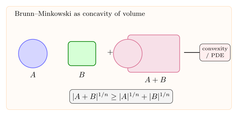
Brunn-Minkowski 不等式：集合加法、离散化与几何 PDE 的影子 — Brunn-Minkowski 不等式说明 Minkowski 加法下体积的 $1/n$ 次方具有凹性。

1. 经典陈述

给定 $\mathbb R^n$ 中的可测集合 $A,B$，定义 Minkowski 和

$$A+B=\{a+b:a\in A,\ b\in B\}.$$

Brunn-Minkowski 不等式说

$$|A+B|^{1/n}\ge |A|^{1/n}+|B|^{1/n}.$$

也可以写成插值形式：对 $0

$$|(1-t)A+tB|^{1/n}\ge (1-t)|A|^{1/n}+t|B|^{1/n}.$$

所以体积的 $1/n$ 次方在集合加法下是凹的。

2. 为什么这个不等式重要

它直接推出等周不等式，也连接到 Prékopa-Leindler 不等式、凸体理论和最优输运。对几何分析来说，更重要的是它提供了一种模板：几何对象的“混合”如果存在，那么与之对应的体积、容量或能量往往应该满足某种凹性。

这正是完全非线性椭圆方程中常见的结构。很多正则性问题并不只是局部估计问题，也和底层几何量的凹性有关。

3. 离散化视角

一种直观证明路线是把集合近似成小立方体的并。连续体积问题被转成格点集合的加法问题。最简单的一维模型是 Cauchy-Davenport 型不等式：

$$|A+B|\ge |A|+|B|-1.$$

这个不等式说明，集合加法至少应该增加自由度。高维情形不能天真地照搬，因为很细的集合可能集中在低维方向上，边界和体积也不再同步。正是这些失败之处提示我们：Brunn-Minkowski 真正使用的是凸化、投影和切片结构。

4. 凸化与测度证明

另一路线是先归约到凸体，再用切片或 Prékopa-Leindler 思想证明。Prékopa-Leindler 可以看成函数版本的 Brunn-Minkowski：如果

$$h((1-t)x+ty)\ge f(x)^{1-t}g(y)^t,$$

那么

$$\int h\ge \left(\int f\right)^{1-t}\left(\int g\right)^t.$$

这说明 Brunn-Minkowski 不只是集合命题，也是积分、概率和凸性之间的共同结构。

5. Hamiltonian 或 level-set 方向的问题

一个自然的问题是：如果我们有一个能量函数 $H$，它的 level sets 形成某种 foliation，并且梯度流或 Hamiltonian flow 在这些 level sets 上诱导出合理的“加法”，是否存在对应的 Brunn-Minkowski 型不等式？

在欧氏空间中，level set 的平移和集合加法非常明确；在一般几何背景中，加法结构可能来自群作用、Hamiltonian flow 或某种可交换的 transport。若这样的不等式成立，它很可能对应某个完全非线性椭圆方程的存在性或正则性。

所以经典 Brunn-Minkowski 在这里扮演的是 toy model：先弄清楚体积凹性怎样从线性加法中出现，再问类似结构能否在更复杂的几何流中重现。

Brunn-Minkowski 不等式：集合加法、离散化与几何 PDE 的影子

旧博客原文

补充说明

1. 经典陈述

2. 为什么这个不等式重要

3. 离散化视角

4. 凸化与测度证明

5. Hamiltonian 或 level-set 方向的问题

更多文章

从支撑接触到 Hausdorff 分层：凸 k-Hessian 解的四步证明机制

From Sum-Free Sets to Strongly 2-Primitive Sets: Localization, Patching, and the Search for Stability

[后端同步测试] 富媒体、代码与数学公式渲染

1