伪微分算子与奇异积分：从 Fourier multiplier 到 symbol calculus

旧博客原文

原题：Pesudo differential opertor and singular integral

I already understand this material 3days ago but it is a little difficult for me to type the latex…

1. Introduction

There is two space to understand a function’s behaviour, the physics space and the frequency space (Why thing going like this? Why there is such a duality?). Namely, we have:

$\displaystyle \hat f(\xi)=\int_{{\mathbb R}^d}e^{2\pi i\xi x}f(x)dx \ \ \ \ \ (1)$

The key point is, waves is a parameter group of scaling of definition of a constant fraquence wave, so it connected the multiplication and addition. Basically due to it can be look as the correlation of a function and the scaling of wave with carry all the information about ${f}$ . A generation of this obeservation is the wavelet theory.

So as we well know, the key ingredient of Fourier transform is to image function as a sum of series waves. A famous theorem of Mikhlion said that a translation-invariant operator ${T}$ on ${R^n}$ could be represented by a multiplication operator on the Fourier transform side. translation is the meaning, ${h\circ T=T\circ h, \forall h}$ is a translation.

In a formal level, consider it as distribution (compact distribution or temperature distribution is both OK). We have:

$\displaystyle T(e^{2\pi ix\xi})=a(\xi)e^{2\pi ix\xi}, \forall \xi \in {\mathbb R}^n \ \ \ \ \ (2)$

the meaning is if we consider ${T}$ is a operator on distribution space, ${T:S'\rightarrow S'}$ , then ${\forall f\in S}$ ,

$\displaystyle \int T(e^{2\pi ix\xi})f=\int a(\xi)e^{2\pi ix\xi}f$

due to the linear combination of ${e^{2\pi ix\xi}}$ will consititue a dense set in ${S}$ . So this could extend to the whole distribution space by dual and give the definition of ${T}$ , i.e.

$\displaystyle (Tf)(x)=\int_{{\mathbb R}^n}a(x,\xi)e^{2\pi ix\xi}\hat f(\xi)d\xi \ \ \ \ \ (3)$

Remark 1 ${T}$ is bounded on ${L^2({\mathbb R}^n)}$ when ${a}$ is a bounded function, thanks to Parevel theorem. When ${a}$ is a bounded function, the composition of two such operator could be defined, and the symbol of composition operator corresponding to the composite of their symbol, i.e.

$\displaystyle T_a\circ T_b(e^{2\pi ix\xi})=b(\xi)a(\xi)e^{2\pi ix\xi} \ \ \ \ \ (4)$

Remark 2 For parenval theorem, i.e. ${\|\hat f\|_2=\|f\|_2}$ , there is two approach, heat kernel approximation approach and discretization.

We wish to investigate the operator given by multiplier, i.e.

$\displaystyle (Tf)(x)=\int_{{\mathbb R}^n}a(x,\xi)e^{2\pi ix\xi}\hat f(\xi)d\xi \ \ \ \ \ (5)$

When it is satisfied ${\|T\|_{p-p}<\infty}$ ?

Intuition, the following calculate is only morally true, not rigorous.

$\displaystyle \begin{array}{rcl} \|Tf\|^p_p & = & \int_{{\mathbb R}^d }|\int_{{\mathbb R}^d}a(x,\xi) e^{2\pi ix\xi} \hat f(\xi)d\xi|^pdx \\ & \overset{\exists f}\sim & \int_{{\mathbb R}^d }\int_{{\mathbb R}^d}|a(x,\xi) e^{2\pi ix\xi} \hat f(\xi)|^p d\xi dx \\ & \overset{Fubini}\sim & \int_{{\mathbb R}^d}\int_{{\mathbb R}^d}|\widehat{a(x,\xi)}\hat f(\xi) |^pdxd\xi \\ & \sim & \int_{{\mathbb R}^n}\int_{{\mathbb R}^n}|{a(x,\xi)}^{\vee}*f(\xi)|^pdxd\xi \end{array}$

So we need some restriction on ${ {a(x,\xi)}^{\vee}}$ , namely ${\widehat{a(x,\xi)}}$ , so we need some decay condition on ${|\partial_x^{\alpha}\partial_{\xi}^{\beta}a(x,\xi)|}$ , why this, just consider integral by part for ${a(x,\xi)\in S}$ . The rigorozaton of this intuition inspirit us to the definition of symbol calss.

Definition 1 we say ${a(x,\xi)}$ is in symbol class ${S_m}$ iff,

$\displaystyle |\partial_x^{\beta}\partial_{\xi}^{\alpha}a(x,\xi)|\leq A_{\alpha,\beta}(1+|\xi|)^{m-|\alpha|} \ \ \ \ \ (6)$

for all ${\alpha,\beta}$ is multi-indece.

Remark 3

we note that all partial differential operator, whose coefficient, together with all their derivatives are bounded belong to this class, In this particular circumstance, the symbol is a polynomial in ${\xi}$ , essentially the “characteristic polynomial” of the operator.

The general operator of this class have a parallel description in terms of their kernels. That is, in a suitable sense,
$\displaystyle (Tf)(x)=\int_{{\mathbb R}_x}K(x,y)f(y)dy \ \ \ \ \ (7)$

besides enjoying a cancellation property, ${K}$ is here characterized by differential inequalities “dual” to those for ${a(x,\xi)}$ . In the key case where the order ${m=0}$ , this kernel representation makes ${T}$ a singular integral operator.

The crucial ${L^2}$ estimate, when ${m=0}$ , is atelatively simple consequences of Plancherel’s theorem for the Fourier transform. With this, the ${L^p}$ theory introduce in previous note is therefore applicable.

The product identity that holds in the translation-invariant case generalized to the situation treated here as a symbolic calculus for the composition of operators. That is, there is an asymptotic formula for the composition of two such operators, whose main term is the point-wise product of their symbols.

The succeeding terms of the formula are of decreasing orders. These orders measure not only the size of the symbols, but determine also the increasing smoothing properties of the corresponding operators. The smoothing properties are most neatly expressed in terms of the Sobolev space ${W_k^p}$ and the Lipschitz space ${\Lambda_{\alpha}}$ .

2. Pseudo-differential operator

“Freezing principle”: from variable coefficient differential equation to constant coefficient differential equation by approximation. divide into 2 steps:

divide space into small cubes.
take average of the coefficient of differential equation in every cubes.

Suppose we are interested in study the solution of the classical elliptic second order equation.

$\displaystyle (Lu)(x)=\sum a_{ij}(x)\frac{\partial^2 u(x)}{\partial x_i\partial x_j}=f(x) \ \ \ \ \ (8)$

Where the coefficient matrix ${\{a_{ij}(x)\}}$ is assume to be real, symmetric, positive definite and smooth in ${X}$ . Understanding ${P}$ , such that,

$\displaystyle PL=I \ \ \ \ \ (9)$

Looking for a ${P}$ . Such that ${PL=I+E}$ . ${E}$ is a error term which have good control. To do this, fix an arbituary point ${x_0}$ , freeze the operator ${L}$ at ${x_0}$ :

$\displaystyle L_{x_0}=\sum a_{ij}(x_0)\frac{\partial^2}{\partial x_i\partial x_j} \ \ \ \ \ (10)$

In Fourier sense ( ${L^2}$ sence).

$\displaystyle \begin{array}{rcl} L_{x_0}f(x) & = & \int e^{2\pi ix\xi}(\widehat{ \sum a_{ij}(x_0)\frac{\partial^2 f(\xi)}{\partial x_i\partial x_j}}) d\xi\\ & = & \int e^{2\pi ix\xi}\int e^{-2\pi i \xi y}\sum a_{ij}(x_0)\frac{\partial^2}{\partial x_i\partial x_j}f(y)dyd\xi\\ & = & \int e^{2\pi ix\xi}(-4 \pi^2)\sum_{i,j}a_{ij}(x_0)\xi_i\xi_j \end{array}$

Remark 4 The remark is, morally speaking, for application of fourier transform in PDE. morally we could only solve the problem with linear differential equation (although we could consider the hyperbolic type). The main obstacle for Fourier transform application into PDE:

it only make sense with Schwarz class or its dual, this is not main obstacle, in principle could be solved by rescaling.

the main obstacle is it only compatible with linear differential equation.

Cut-off function: ${\eta}$ vanish near the origin,

$\displaystyle (P_{x_0}f)=\int_{{\mathbb R}^n}(-4\pi^2\sum_{i,j}a_{ij}(x_0)\xi_i\xi_j)^{-1}\eta(\xi)\hat {f(\xi)}e^{2\pi ix\xi}d\xi. \ \ \ \ \ (11)$

then:

$\displaystyle L_{x_0}P_{x_0}=I+E_{x_0}.$

${E_{x_0}}$ is actually a smoothing operator, because it is given by convolution with a fixed test function. It should be seasonable when ${x}$ near ${x_0}$ , ${(Pf)(x)}$ is well approximated by ${(P_{x_0}f)(x)}$ , it is actually the case, define ${((Pf)(x):=(P_xf)(x)}$ , i.e.

$\displaystyle (Pf)(x)=\int_{{\mathbb R}^n}(-4\pi^2\sum_{i,j}a_{ij}(x)\xi_i\xi_j)^{-1}\eta(\xi)\hat f(\xi)e^{2\pi ix\xi}d\xi \ \ \ \ \ (12)$

The operator ${P}$ so given is a propotype of a pesudo-differential operator. Moreover, one has ${LP=I+E}$ , where the error operator ${E}$ is “smoothing of order 1”. That this is indeed the case is the main part of the symbolic calculus described.

Definition 2 (symbol class) A function ${a(x,\xi)}$ belong to ${S^m}$ and is said to be of order ${m}$ of ${a(x,\xi)}$ is a ${C^{\infty}}$ function of ${(x,\xi)\in {\mathbb R}^n\times {\mathbb R}^n}$ and satisfies the differential inequality:

$\displaystyle |\partial_x^{\beta}\partial_{\xi}^{\alpha}a(x,\xi)|\leq A_{\alpha,\beta}(1+|\xi|)^{m-|\alpha|} \ \ \ \ \ (13)$

For all ${\alpha,\beta}$ are multi-indece.

Now we trun to the exact meaning of pesudo-differential operator, i.e. how them action on functions. Under some suffice given regularity condition, for ${a\in S^m}$ , ${T_a:S\rightarrow S}$ .

$\displaystyle (Tf)(x)=\int_{{\mathbb R}^n}a(x,\xi)\hat f(\xi)e^{2\pi ix\xi}d\xi \ \ \ \ \ (14)$

Remark 5 ${T_a:S\rightarrow S}$ is continuous and for ${a_k\rightarrow a}$ pointwise, ${a_k\in S,\forall k\in {\mathbb N}^*}$ , ${T_{a_k}(f)\rightarrow T_a(f)}$ in ${S}$ .

then expense it, we get:

$\displaystyle (T_af)(x)=\int\int a(x,\xi)e^{2\pi i\xi(x-y)}f(y)dyd\xi \ \ \ \ \ (15)$

This could be diverge, even when ${f\in S}$ . The key point is we do not have control with the second integral, morally speaking, this phenomenon is the weakness of Lesbegue integral which would not happen in Riemann integral, so sometime we need the idea from Riemann integral, this phnomenon is settle by multi a cut off function ${\eta_{\epsilon}}$ and take ${\epsilon\rightarrow \infty}$ , the same deal also occur as the introduced of P.V. integral in Hilbert transform. The precise method to deal with the obstacle is following: ${a_{\epsilon}(x,\xi)=a(x,\xi)\gamma(\epsilon x,\epsilon \xi)}$ , if ${a\in S^m}$ , ${a_{\epsilon}\in S^m}$ . ${T_{a_{\epsilon}}\rightarrow T_a}$ in the sense:

${\forall f\in S}$ , ${T_{a_{\epsilon}}(f)\rightarrow T_a(f)}$ ,

$\displaystyle (T_af)(x)=\lim_{\epsilon\rightarrow 0}\int\int a_{\epsilon}(x,\xi)e^{2\pi i\xi(x-y)}f(y)dyd\xi \ \ \ \ \ (16)$

We also have:

$\displaystyle <T_af,g>=<f,T_a^*g>, \forall f,g\in S. \ \ \ \ \ (17)$

Then we have:

$\displaystyle (T^*_ag)(y)=\lim_{\epsilon\rightarrow 0}\int\int \bar a_{\epsilon}(x,\xi)e^{2\pi i\xi(y-x)}g(x)dxd\xi \ \ \ \ \ (18)$

and ${<f,g>}$ denotes ${\int_{{\mathbb R}^n}f(x)\bar g(x)dx}$ . Thus the pesudo-differential operator ${T_a}$ initially defined as a mapping from ${S}$ to ${S}$ , extend via the identity 17 to a mapping from the space of temperatured distribution ${S'}$ to itself ${S'}$ . Notice also that ${T_a}$ is automatically continuous in this space. \newpage

3. ${L^p}$ bounded theorem

We first introduce a powerful tools, called dyadic decomposition,

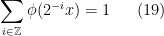
Lemma 3 (dyadic decomposition) In eculid space ${{\mathbb R}^n}$ there exists a function ${\phi\in C^{\infty}({\mathbb R}^n)}$ such that,

$\displaystyle \sum_{i\in {\mathbb Z}}\phi(2^{-i}x)=1 \ \ \ \ \ (19)$

and ${\forall x\in {\mathbb R}^n}$ , there is only two of ${i\in {\mathbb Z}}$ such that ${\phi(2^{-i}x)\neq 0}$ , and we can choose ${\phi}$ to be radical and ${\phi(x) \geq 0,\forall x\in {\mathbb R}^n}$ .

Remark 6

So for a given mutiplier ${a(x,\xi)}$ , we will have ${a(x,\xi)=\sum_{i\in {\mathbb Z}}a_i(x,\xi)=\sum_{i\in Z}\phi(2^{-ix})a(x)}$ .

Proof: The proof is easy, after rescaling we just need observed there is a bump function satisfied whole condition. $\Box$

Theorem 4 Suppose ${a}$ is a symbol of order 0, i.e. that ${a\in S^0}$ Then the operator ${T_a}$ , initially defined on ${S}$ , extends to a bounded operator from ${L^2({\mathbb R}^n)}$ to itself.

Remark 7 Suffice to show ${\|T_a(f)\|_{L^2}\leq A\|f\|_{L^2}, \forall f\in S}$ and by dual.

In fact we can directly proof a more general theorem:

Theorem 5 Let ${m:{\mathbb R}^d-\{0\}\rightarrow {\mathbb C}}$ satisfy, for any multi-index ${\gamma}$ of length ${|\gamma|\leq d+2}$ ,

$\displaystyle |\partial^{\gamma}m(\xi)|\leq B|\xi|^{-|\gamma|}$

For all ${\xi\neq 0}$ . Then, for any ${0<p<\infty}$ , there is a constant ${C=C(d,p)}$ such that,

$\displaystyle \| (m\hat f)^{\vee}\|_p\leq C(p,d)\|f\|_p \ \ \ \ \ (20)$

for all ${f\in S}$ .

Proof: ${a\in S^0}$ , so we have:

$\displaystyle |\partial_x^{\beta}\partial_{\xi}^{\alpha}a(x,\xi)\leq a_{\alpha,\beta}(1+|\beta|)^{-|\alpha|} \ \ \ \ \ (21)$

${\forall \alpha,\beta}$ are multi indeces. Then we consider dyadic decomposition, the is a function ${\phi}$ satisfied the condition in 19, define ${a_i(x,\xi)=\phi(2^{-i}x)a(x)}$ . then ${supp a_i(x,\xi)}$ cpt, ${\|a_i\|<\infty}$ . So ${a_i\in L^p({\mathbb R}^n)}$ , we have,

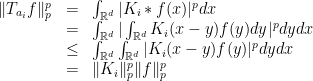
$\displaystyle \begin{array}{rcl} \|T_{a_i}f\|_p^p & = & \int_{{\mathbb R}^d}|K_i*f(x)|^pdx \\ & = & \int_{{\mathbb R}^d}|\int_{{\mathbb R}^d}K_i(x-y)f(y)dy|^pdydx\\ & \leq &\int_{{\mathbb R}^d}\int_{{\mathbb R}^d}|K_i(x-y)f(y)|^pdydx\\ & = & \|K_i\|_p^p\|f\|_p^p \end{array}$

${\|K_i\|_p}$ have good decay estimate, thanks to ${u_i=\phi(2^{-i}x)a(x)\in S^0}$ , this estimate is deduce morally along the same ingredient of “station phase”, it is come from a argument combine “counting point” argument and a rescaling argument. So,

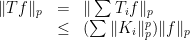
$\displaystyle \begin{array}{rcl} \|Tf\|_p & = & \|\sum T_if\|_p\\ & \leq & (\sum \|K_i\|_p^p)\|f\|_p \end{array}$

But we have ${\sum\|K_i\|_p^p\leq \infty}$ , ending the proof. $\Box$

Remark 8 this method also make sense of restrict the condition to be:

$\displaystyle |\partial_x^{\beta}\partial_{\xi}^{\alpha}a(x,\xi)|\leq A_{\alpha,\beta}(1+|\xi|)^{-|\alpha|}, \forall |\alpha|\leq d+2. \ \ \ \ \ (22)$

Where ${d}$ is the dimension of the space, and we could change ${2}$ to ${1+\epsilon}$ .

Remark 9

$\displaystyle \widehat{\frac{\partial^2 u}{\partial x_i\partial x_j}}|\xi|=\frac{\xi_i\xi_j}{|\xi|^2}\widehat \Delta u(\xi), m(\xi)=\frac{\xi_i\xi_j}{|\xi|^2} \ \ \ \ \ (23)$

is a counter example for ${p=1,\infty}$ .

Remark 10 The key point is the estimate

$\displaystyle \int|\int e^{2\pi i\xi x}\phi(2^{-j}\xi)m(\xi)d\xi |^pdx \ \ \ \ \ (24)$

Correlation of taylor expension and wavelet expension. This is also crutial for the theory of station phase.

4. Calculus of symbols

This calculus of symbols would imply there is some structure on this set.

Theorem 6 Suppose ${a,b}$ are symbols belonging to ${S^{m_1}}$ and ${S^{m_2}}$ respectively. Then there is a symbol ${c}$ in ${S^{m_1+m_2}}$ so that:

$\displaystyle Tc=T_a\circ T_b$

Moreover,

$\displaystyle c\sim \sum_{\alpha}\frac{(2\pi i)^{-|\alpha|}}{\alpha}(\partial_{\xi}^{\alpha}a)(\partial_x^{\alpha}b). \ \ \ \ \ (25)$

in the sense that,

$\displaystyle c-\sum_{|\alpha|<N}\frac{(2\pi i)^{-|\alpha|}}{\alpha !}\partial_{\xi}^{\alpha}\partial_x^{\alpha}b\in S^{m_1+m_2-N} \ \ \ \ \ (26)$

For all ${N>0}$ .

The following “proof” is not rigorous, we just calculate it formally, we could believe it is true rigorously, by some approximation process. Proof: We assume ${a,b}$ have compact support so that our manipulations are justified. We use the alternate formula 15 to write,

$\displaystyle (T_af)(y)=\int b(y,\xi)e^{2\pi i\xi(y-z)}f(z)dzd\xi \ \ \ \ \ (27)$

Then we apply ${T_a}$ , again in the form 15, but here with the variable ${\eta}$ replacing in the integration. The result is,

$\displaystyle T_a(T_bf)(x)=\int a(x,\eta)b(y,\xi)e^{2\pi i\eta(x-y)}e^{2\pi i\xi(y-z)}f(z)dzd\xi dyd\eta. \ \ \ \ \ (28)$

This calculate is easy to derive, but the following is more tricky. Now ${e^{2\pi i\eta(x-y)}\cdot e^{2\pi i\xi(y-z)}=e^{2\pi i(x-y)(\eta-\xi)}\cdot e^{2\pi i(x-z)\xi}}$ , so

$\displaystyle T_a(T_bf)(x)=\int c(x,\xi)e^{2\pi i(x-z)\xi}f(z)dz d\xi \ \ \ \ \ (29)$

with

$\displaystyle c(x,\xi)=\int a(x,\eta)b(y,\xi)e^{2\pi i(x-y)(\eta-\xi)}dyd\eta \ \ \ \ \ (30)$

we can also carry out the integration in the y-variable. This leads to the corresponding Fourier transform of ${b}$ in that variable, and allows us to rewrite 30 as,

$\displaystyle c(x,\xi)=\int a(x,\xi+\eta)\hat b(\eta,\xi)e^{2\pi i x\eta}d\eta. \ \ \ \ \ (31)$

With this form in hand, use taylor expense to the symbol ${a(x,\xi+\eta)}$ , i.e.

$\displaystyle a(x,\xi+\eta)=\sum_{|\alpha|<N}\partial_{\xi}^{\alpha}a(x,\xi)\eta^{\alpha}+R_N(x,\xi,\eta) \ \ \ \ \ (32)$

with a suitable error term ${R_N}$ , due to

$\displaystyle \frac{1}{\alpha !}\int \partial_{\xi}^{\alpha}a(x,\xi)\hat\eta(\eta,\xi)e^{2\pi ix\eta}d\eta=\frac{(2\pi i)^{|\alpha|}}{\alpha !}(\partial_{\xi}^{\alpha}a(x,\xi))(\partial_x^{\alpha}b(x,\xi)). \ \ \ \ \ (33)$

we only need to proof ${R_N\in S^{m_1+m_2-N}}$ and it is definitely the case, we get the theorem. $\Box$

Remark 11 We need replace ${a,b}$ with ${a_{\epsilon},b_{\epsilon}}$ , where

$\displaystyle a_{\epsilon}(x,\xi)=a(x,\xi)\cdot \gamma(\epsilon ,\epsilon \xi), b_{\epsilon}(x,\xi)=b(x,\xi)\cdot \gamma(\epsilon ,\epsilon \xi). \ \ \ \ \ (34)$

we note that ${a_{\epsilon},b_{\epsilon}}$ satisfy the same differential inequalities that ${a}$ and ${b}$ do, uniformly in ${\epsilon, 0<\epsilon\leq 1}$ .passage to the limit as ${\epsilon\rightarrow 0}$ will then give us our desired result.

5. Estimate in ${L^p}$ , Sobolev, and Lipchitz space

We now take up the regularity properties of our pesudo-differential operator as expressed in terms of the standard function spaces, we begin with the ${L^p}$ boundedness of an operator of order ${0}$ .

5.1. ${L^p}$ estimate

Suppose ${a}$ belongs to the symbol class ${S^0}$ . Then, we can express ${T=T_a}$ as

$\displaystyle (Tf)(x)=\int K(x,y)f(y)dy=\int K(x,x-y)f(y)dy \ \ \ \ \ (35)$

due to ${a\in S^0}$ , we know, with some approximation argument and first do it with a cutoff symbol of ${a}$ , i.e. ${a_{\epsilon}}$ , that,

$\displaystyle |K(x,y)|\leq A|x-y|^{-n} \ \ \ \ \ (36)$

So that the integral coverage whenever ${f\in S}$ and ${x}$ is away from the support of ${f}$ . Since we know that ${T}$ is bounded on ${L^2({\mathbb R})}$ , this representation extends to all ${f\in L^2({\mathbb R})}$ for almost every ${x\notin supp f}$ . More generally, we have,

$\displaystyle |\partial_{x}^{\alpha}\partial_{y}^{\beta}K(x,y)|\leq A_{\alpha,\beta}|x-y|^{-n-|\alpha|-|\beta|} \ \ \ \ \ (37)$

hence ${K}$ satisfies,

$\displaystyle \int_{|x-y|\geq 2\delta}|K(x,y)-K(x,\bar y)|dx\leq A, \ if\ |y-\bar y|\leq \delta, all \ \ \delta>0. \ \ \ \ \ (38)$

Use the general singular integral theory we get the following ${L^p}$ estimate.

Theorem 7 Suppose ${T_a}$ is the pseudo-differential operator corresponding to a symbol ${a}$ in ${S^0}$ , then ${T_a}$ extends to a bounded operator on ${L^p({\mathbb R}^n)}$ to itself, for ${1<p<\infty}$ .

5.2. Sobolev spaces

We first recall the definition of the Sobolev spaces ${W_k^p}$ , where ${k}$ is a positive integer. A function ${f}$ belongs to ${W_k^p({\mathbb R}^n)}$ if ${f\in L^p({\mathbb R}^n)}$ and the partial derivatives ${\partial_x^{\alpha}f}$ , taken in the sense of distribution, belong to ${L^p({\mathbb R}^n)}$ , whenever ${0\leq |\alpha|\leq k}$ . The norm in ${W_k^p}$ is given by,

$\displaystyle \|f\|_{W_k^p}=\sum_{|\alpha|\leq k}\|\partial_x^{\alpha}f\|_{L^p} \ \ \ \ \ (39)$

the following result is the directly corollary of 7.

Theorem 8 Suppose ${T_a}$ is a pseudo-differential operator whose symbol ${a}$ belongs to ${S^m}$ . If ${m}$ is an integer and ${k\geq m}$ , then ${T_a}$ is a bounded mapping from ${W_k^p}$ to ${W_{k-m}^p}$ , whenever ${1<p<\infty}$ .

Remark 12 This theorem remain valid for arbitrary real ${k,m}$ .

5.3. Lipschitz spaces

Theorem 9 Suppose ${a}$ is a symbol in ${S^m}$ . Then the operator ${T_a}$ is a bounded mapping from ${\Lambda_{\gamma}}$ to ${\Lambda_{\gamma-m}}$ , whenever ${\gamma>m}$ .

Lemma 10 Suppose the symbol ${a}$ belongs to ${S^m}$ , and define ${T_{a_j}=T_a\Delta_j}$ . Then, as operator from ${\L^{\infty}({\mathbb R}^n)}$ to itself, the ${T_{a_j}}$ have norms that satisfy

$\displaystyle \|T_{a_j}\|\leq A2^{jm} \ \ \ \ \ (40)$

We shall now point out a very simple but useful alternative characterization of ${\Lambda_{\gamma}}$ . This is in terms of approximation by smooth functions; it is also closely connected with the definition of ${\Lambda_{\alpha}}$ space as intermediate spaces, using the “real” method of interpolation.

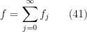
Corollary 11 A function ${f}$ belongs to ${\Lambda_{\gamma}}$ if and only if there is a decomposition,

$\displaystyle f=\sum_{j=0}^{\infty}f_j \ \ \ \ \ (41)$

with ${\|\partial_x^{\alpha}f_j\|_{L^infty}\leq A2^{-j\gamma}\cdot 2^{j|\alpha|}}$ , for all ${0\leq |\alpha|\leq l}$ , where ${l}$ is the smallest integer ${>\gamma}$ .

When ${f\in \Lambda_{/\gamma}}$ , the argument prove 10, with ${T_a=I}$ , ${f_j=F_j=\Delta_j(f)}$ , gives the required estimate for the ${f_j}$ .

A second consequence of 9 is the following:

Corollary 12 The operator ${(I-\Delta)^{\frac{m}{2}}}$ gives an isomorphism from ${\Lambda_{\gamma}}$ to ${\Lambda_{\gamma-m}}$ , whenever ${\gamma>m}$ .

This is clear because ${(I-\Delta)^{\frac{m}{2}}}$ is continuous from ${\Lambda_{\gamma}}$ to ${\Lambda_{\gamma-m}}$ , and its inverse, ${(I-\Delta)^{\frac{-m}{2}}}$ , is continuous from ${\Lambda_{\gamma-m}}$ to ${\Lambda_{\gamma}}$ .

补充说明

以下是新整理的中文说明；上方旧博客原文保持不变。

理解伪微分算子的一个自然入口，是先理解 Fourier multiplier。平移不变算子在频率侧通常只是乘以一个函数；一旦系数依赖空间位置，乘子就必须升级为同时依赖 $x$ 和 $\xi$ 的 symbol。这篇笔记沿着这个想法，从 multiplier 走到 kernel，再走到 Calderon-Zygmund 型奇异积分。

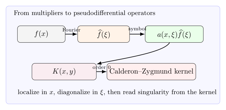
伪微分算子与奇异积分：从 Fourier multiplier 到 symbol calculus — 伪微分算子把位置变量 $x$ 和频率变量 $\xi$ 同时放进 symbol，kernel 的奇异性由 symbol 的阶数控制。

1. Fourier multiplier

若 $T$ 与平移可交换，那么在 Fourier 侧它应当满足

$$\widehat{Tf}(\xi)=m(\xi)\widehat f(\xi).$$

这里 $m$ 是 multiplier。Plancherel 定理直接给出一个基本结论：如果 $m\in L^\infty$，那么 $T$ 在 $L^2$ 上有界，并且

$$\|Tf\|_2\le \|m\|_\infty\|f\|_2.$$

这解释了为什么频率空间是处理常系数线性方程的自然语言：微分在频率侧变成乘法，算子代数变成函数代数。

2. 从 multiplier 到 symbol

变系数方程的困难在于，算子不再平移不变。伪微分算子的基本形式是

$$Af(x)=\int_{\mathbb R^n}e^{ix\cdot\xi}a(x,\xi)\widehat f(\xi)\,d\xi.$$

函数 $a(x,\xi)$ 称为 symbol。它描述算子在点 $x$ 附近、频率 $\xi$ 方向上的局部行为。常系数情形是 $a$ 不依赖 $x$ 的特例。

标准 symbol class $S^m_{1,0}$ 要求对所有多重指标 $\alpha,\beta$，有

$$|\partial_x^\alpha\partial_\xi^\beta a(x,\xi)|\le C_{\alpha\beta}(1+|\xi|)^{m-|\beta|}.$$

对 $\xi$ 求导会降低阶数，这正对应物理空间 kernel 的衰减和光滑性。

3. Freezing principle

变系数椭圆方程可以先在一个点附近“冻结系数”。例如二阶椭圆算子

$$Lu=-\partial_i(a^{ij}(x)\partial_j u)$$

在点 $x_0$ 附近可以用常系数算子

$$L_{x_0}u=-a^{ij}(x_0)\partial_i\partial_j u$$

作为第一近似。Fourier transform 可以求解冻结后的模型；误差则由系数的变化控制。伪微分算子把这个“每个点冻结一次”的过程系统化了。

4. Kernel 与奇异积分

伪微分算子也可以写成 kernel 形式

$$Af(x)=\int K(x,y)f(y)\,dy.$$

当 symbol 的阶数 $m=0$ 时，kernel 在 $x=y$ 附近有奇异性，但又满足 cancellation 和光滑估计。这就把问题接到 Calderon-Zygmund 理论：$L^2$ 有界性来自 Plancherel，弱 $(1,1)$ 或 $L^p$ 有界性则依赖实变量分解。

因此，伪微分算子不是孤立的一套语言，而是 Fourier 分析和实变量奇异积分之间的桥。

5. Symbolic calculus

平移不变情形下，两个 multiplier 的复合对应乘子相乘。伪微分算子也有类似结论，只是要加入低阶修正。形式上，如果 $A$ 的 symbol 是 $a$，$B$ 的 symbol 是 $b$，那么 $AB$ 的 symbol 有渐近展开

$$a\# b(x,\xi)\sim \sum_\alpha \frac1{\alpha!}\partial_\xi^\alpha a(x,\xi)D_x^\alpha b(x,\xi).$$

主项是 $ab$，后面的项阶数越来越低，表示越来越强的 smoothing。这个公式是椭圆正则性、参数构造和微局部分析的基本计算规则。

伪微分算子与奇异积分：从 Fourier multiplier 到 symbol calculus

旧博客原文

补充说明

1. Fourier multiplier

2. 从 multiplier 到 symbol

3. Freezing principle

4. Kernel 与奇异积分

5. Symbolic calculus

更多文章

从支撑接触到 Hausdorff 分层：凸 k-Hessian 解的四步证明机制

From Sum-Free Sets to Strongly 2-Primitive Sets: Localization, Patching, and the Search for Stability

[后端同步测试] 富媒体、代码与数学公式渲染

1