I post two problem here, this is a product due to a random walk along the boundary of topology and the analysis,
Problem 1.
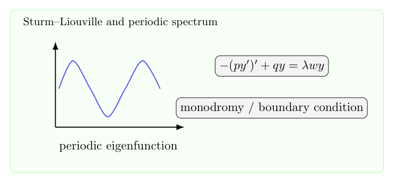
Fix a set , is there a 2 order ordinary differential equation given by Sturm–Liouville theory such that the eigenfunction is periodic if and only if ?
There is also some weak version of this and a infinity version of this.
Of course we have the following map, from the high order ordinary differential equation to the 1 order differential equation in high dimension. But the key point is that it is not a bijection! The Frobenius condition play a crucial role.
Problem 2.
There is a homotopy in the moduli space of differential equation, and we could define a direct product operator in this space, and we consider the topology defamation of the eigenfunction, could there be some equality, one side of it explain the topology information, the other side explain the spectral (or analysis) information?
We focus on , it does not mean is the only compact 1 dimensional system , but it is a typical example.
.
If is a homomorphism then stay the order of (by continuous and the zero point theorem). That is just mean:
(may be do a reflexion ).
In the homomorphism case. We try to define the rotation number to describe the expending rate of the dynamic system.
i.e. . Lifting to,
.
How to realize the lifting?
Step1: Periodic extend to . (Regard as ).
Step2: Consider the “flow” of . we get .
The rotation number is defined as:
.
Following we will shall it is independent of the choice of and in fact.
It is not difficult to proved the following property:
Property:
1.If is conjugate (in fact semi-conjugate is enough ). Then 1.If is conjugate (in fact semi-conjugate is enough ). Thenrotation number of equal to rotation number of .
2.If is conjugate to . Then rotation number of equal to
rotation number of .
)
Example: , . It is not difficult to prove the rotation number of is .
Propersion:
1)For we have that .
2).If has a periodic point, i.e. . Then $latex\rho (T)$ is rational.
3) has no periodic point then is irrational.
4) The limit actually exists and we have: .
pf of 1):
.
Used the property .
pf of 2):
It is not difficult to prove is independent with the choice of . So choose to be the periodic point.
Remark: but the inverse of 2) is not true. For example:
.
This dynamic system has both periodic points() and non-periodic pint (maybe orbits generated by .
pf of 3):
If not. Assume is rational number . Take any point , then:
.
.
.
Now assume .
Then . $\forall x\in \mathbb S_1$ (if , take reflection ).
And there do not exists such that . If not, we could prove rotation number is large than lead a contradiction.
So is a bounded monotonically increasing sequences in , it limits point must satisfied .
pf of 4):
Using the point wise approximation inequality induced from the monotonically and stay ordering property of by .
Corollary:
Assume is irrational.
1. Let , and . If , then .
2. The bijection between the set and precise the natural ordering on .
This corollary is not difficult to prove use the established property.
Denjoy’s theorem
Proposition:
If is a minimal orientation presenving homomorphism with irrational rotation number then is topologically conjugate to the standard rotation .
leave as a ex.
For , . We define the variation of by:
We say that the logarithm of has bounded variation if this value is finite.
Denjoy’s theorem:
If is a orientation preserving homomorphism of the circle with derivative of standard variation and irrational rotation number then is topologically conjugate to the standard rotation :
.
Due to the upper proposition we only need show is minimal. Proof pf minimal is splitting to following two sub lemmas.
Sublemma1:
If has irrational rotation number and there are a constant and a sequences of integers such that the map: Satisfy : Then is minimal.
Sublemma2:
Fix and write , for There exists an increasing sequences of natural number such that the intervals are all disjoint.
Paradox and problem
Graph:
because of existence of fix point.
for .
Is always true for ?
If it is right, then there is a contradiction with argument , but for what type of dynamic system ?
satisfied . for all ?
Problem:
If is not homomorphism but induced , is striating increasing, Is the limit of always exists? it could not be increase with .
补充说明
以下是新整理的中文说明;上方旧博客原文保持不变。
rotation number 是一维动力系统中最基本的不变量之一。它衡量圆周同胚平均每次迭代旋转多少。
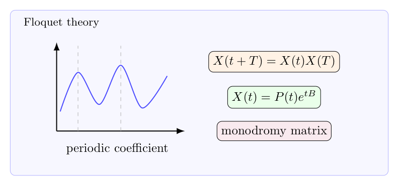
Where is a given periodic matrix with period , i.e. .
Then the solution $\phi(t)$ satisfied identity:
.
This could be explained as .
Now we consider to solve the equation: . At least formally it could be solved:
.
(Unfortunately is a multi-value function so , where is the identity matrix and is a solution of .) This argument is false.
In fact matrix is not like numbers, the function is much more complicated. we have,
So to solve , it is equivalent to :
But this type of identity only meaningful when , so is it true that for the equation is solved by , and for it do not have solution?
The naive inspirit is wrong, the situation is similar to the case while could extend to and the identity
always holds for . The key observation is always holds when , this will lead to a reasonable value of
even when and this process could be continue to the whole matrix space and the identity enjoy the accosted principle so is well-defined for all .
Now it is time to consider the rotation number, which is defined by for is a continuous increasing function.
And I do not know how to associated a dynamic system for the matrix given here, but in any case it seems iff it is given by a hemoermorphifm then the rotation number is zero due to the following reason:
Consider as the quotient . Your homeomorphism lifts to a homeomorphism
such that .
Form the map , where is the composition times of with itself. By construction and , so that factors as a homeomorphism of the circle conjugating to the rotation.
By the way this approach wors in too.
Maslov index of a holomorphic disk
A natural way to understand the rotation number here is according the way of maslov index, we have the following formula:
Proof sketch:
1..
2. The dynamic system is defined by : , .
3. this dynamic system is conjugate to the dynamic system , Not difficult to proof it is a homomorphism on and it is zero entropy by Pesin’s formula
If could lifting to $\hat T:R \to R$ the rotation number is defined as :
This problem is not a good problem due to the philosophy, i.e. use rotation number to describe the information of a hamiltonian flow is not satisfied, in fact it is difficult to establish a suitable definition of “rotation number”! But this is the first crucial thing to establish a theorem!
Hamiltonian flow
In mathematics and physics, a Hamiltonian vector field on a symplectic manifold is a vector field, defined for any energy function or Hamiltonian. A Hamiltonian vector field is a geometric manifestation of Hamilton’s equations in classical mechanics. The integral curves of a Hamiltonian vector field represent solutions to the equations of motion in the Hamiltonian form. The diffeomorphisms of a symplectic manifold arising from the flow of a Hamiltonian vector field are known as canonical transformations in physics and (Hamiltonian) symplectomorphisms in mathematics.[1]
Hamiltonian vector fields can be defined more generally on an arbitrary Poisson manifold. The Lie bracket of two Hamiltonian vector fields corresponding to functions f and g on the manifold is itself a Hamiltonian vector field, with the Hamiltonian given by the Poisson bracket of f and g.
补充说明
以下是新整理的中文说明;上方旧博客原文保持不变。
Floquet theory 研究周期系数线性微分方程
$$\dot x=A(t)x,\qquad A(t+T)=A(t).$$
它告诉我们,周期系统的长期行为由一个周期部分和一个指数部分共同决定。
Floquet theory 把周期系数线性系统分解成周期部分和指数部分,monodromy matrix 控制稳定性。
原题:Sarnak conjecture, understand with standard model
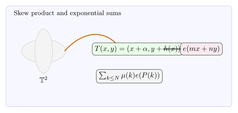
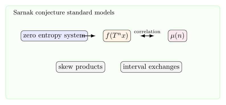
Sarnak conjecture is a conjecture lie in the overlap of dynamic system and number theory. It is mainly focus on understanding the behavior of entropy zero dynamic system by look at the correlation of an observable and the Mobius function .
We state it in a rigorous way:
let be a entropy zero topological dynamic system. Let Mobius function be defined as , where $latex$ is the number of different primes occur in the decomposition of .
Then for any continuous function and , observable is orthogonal to the Mobius function; i.e. ,
by Bourgain-Ziegelar-Sarnak theorem we know the difficulties is focus on deal with the exponent
for all is suffice large primes pair.
and a much simper case is the affine map: on and the general case where A is a upper-triangle matrix with diagonal 1; i.e. , B is nilpotent. So the sarnak conjecture in this case is reduce to the Davenport estimate on exponent by B-Z-S theorem:
, .
Interval exchange map
For the interval exchange map, we can explain it by a composition of rotation of some part of step by step and with a renormalization process to glue the neighbor rotations.
Now let us explain a little with this interesting dynamic system. We focus in the simplest nontrivial case, which is the 3-interval exchange map. In this case, just consider the permutation of intervals , and it is easy to see there is only one case is nontrivial that is permutation: . We explain a little more with other trivial case:
When , the interval exchange map is just a rotation and for which the sarnak conjecture is just come from:
, .
Which is trivial because .
For the case $I_1\to I_2, I_2\to I_1, I_3\to i_3$ the map is a rotation on but it is a identity map on and the orbits of point only lying one of $I_1\cap I_2, I_3$, lying in which one depend on the original point we take is lying in which one.
Now we focus on the most difficult situation. It is annoying but it is the obstacle we must get over to go far. Fortunately it could be explained as in the following picture.
3-Interval exchange map as two rotation map glue with a renormalization map.
Now we explain what happen in the picture, it is mainly say one identity, which explain how to look 3-interval exchange map as a composition of rotation map with a renormalization map to glue them. Rotation is a kind of map we have good understanding but we do not understand very well with the renormalization map which is glue the two endpoints of which are not the common endpoint of them. Then you get two circle glue like a “8” , and is just rotate one of it and make the other one to be invariance.
Now we roughly could think about what is the thing we need to charge with, it is just:
.
Now we do some calculate with this geometric explain of interval exchange map.
Let , then . And , . the rotation , .
Standard model
Is there a standard model of entropy zero dynamic system?
This problem seems to be too ambitious. But it occur naturally when I an trying to have a global understand of the Sarnak conjecture.
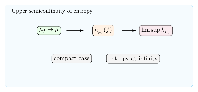
Now we focus on the upper semi-continuouty of the metric entropy map. The object we investigate is , where is a invariant measure.
The insight to make us interested to this kind of problem is a part of variational problem, something about the existence of certain object which combine a certain moduli space to make some quantity attain critical value(maximum or minimum). The most simple example maybe Isoperimetric inequality and Dirichlet principle of Laplace. Any way, to establish such a existence result a classical approach is to proof the upper semi-continuouty and bounded for associate energy of the problem. In our case the semi-continuouty will be some thin about the regularity of the entropy map:
We define the entropy at infinity:
Where varies in all sequences of measure coverage to in the sense for all , measurable then .
Compact case
we say some thing about the compact case, In this case we have finite partition with smaller and smaller cubes, this could be understand as a sequences of smaller and smaller scales. A example to explain the differences is , shift map on countable alphabet.
Because of this thing, there is a good sympolotic model, i.e. h-expension, and it generalization asymptotically h-expension equipped on a compact metric space $X$ have been proved to be that the corresponding entropy map is upper semi-continous.
In particular diffeomorphisms on compact manifold is asymptotically h-expensive.
Natural problem but I do not understand very well:
Why it is natural to assume the measure to be probability measure in the non-compact space?
Non-compact case
metric space
is a continuous map.
, then is still a metric.
Easy to see . This identity could be proved by the cretition of entropy by -seperate set and -cover set.
Kapok theorem:
compact, for every ergodic measure the following formula hold:
.
Where is the measure theoretic entropy of .
Riquelme proved the same formula hold for Lipchitz maps on topological manifold.
Let defined the moduli space of -invariant portability measure.
Let defined the moduli space of ergodic -invariant probability measure.
Simplified entropy formula:
satisfied simplified entropy formula if surfaced small and , .
Some basic thing, include the definition of metric entropy is introduced in my early blog.
Among the other thing, there is something we need to focus on:
1.Definition of metric entropy, and more general, topological entropy.
2.Spanning set and separating set describe of entropy.
3.amernov theorem:
.
Now we state the result of Margulis and Ruelle:
Let be a compact riemannian manifold, is a diffeomorphism and is a -invariant measure.
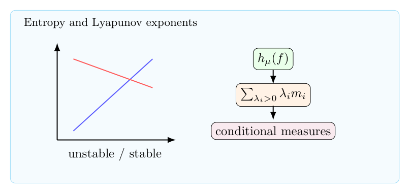
Entropy is always bounded above by the sum of positive exponents;i.e.,
Where is the multiplicity of and .
Pesin show the inequality is in fact an equality if and is equivalent to the Riemannian measure on . So this is also sometime known as Pesin’s formula.
F.Ledrappier and L.S.Young generate the result of Pesin.
One of their main result is:
is a diffemoephism, where is a compact riemanian manifold, f is compatible with the Lesbegue measure on , and
If and only if on the canonical defined quation manifold $M/W_{\mu}$, i.e. the manifold mod unstable manifold $W_{\mu}$, the induced conditional measure is absolute continuous.
Remark: according to my understanding, the equality just mean in some sense we have the inverse estimate:
This result maybe just mean near the fix point of ,i.e. the place charge the topology of the foliation, we have the inverse estimate. Such a inverse estimate will lead a control of the singularity of the push forward measure on the quation manifold. So have good regularity. But this idea is not complete to solve the problem.
Now we begin to get a geometric explain and which will lead a rigorous proof of the inequality:
At first we could observe that the long time average of could be diagonal. Assume after diagonal the eigenvalue is
.
This eigenvalue could divide into 3 parts: <0,=0,>0.
This will lead to a direct sum decomposition of the tangent bundle :
Where $E_u$ is the part corresponding to the eigenvalue>0, For this part we consider the more refinement decomposition:
, is the eigenvector space of . The dimension of $V_k$ is $dim V_k$.
On the other hand, we have a equality of metric entropy:
.
For the later one, is a measurable partition of , then could always be refine to a smaller partition , and we have:
.
Now we arrive the central place of the proof:
every partition could be refine by a partition with boundary of almost all cubes is parallel to the foliation. So we focus ourselves on the portion and all boundary of cubes in is parallel to the eigenvector.
Under this situation, we need only estimate the numbers of . Estimate it is not very difficult. we need only observe the following two thing:
1.
exists a.e. in . So this lead to the definition of foliation almost everywhere, and except a measurable zero set. In fact this set is the set of fix point of under .
2.
After a rescaling, every point which is not a fix point of could be understand as it is far away from fix points. Then the foliation could be understand as a product space locally. The flow with the direction which the eigenvalue is less than 1 cold not change . The direction with eigenvalue equal to 1 is just transition and just change the number of with polynomial growth. But the central thing is the direction with eigenvalue large than one and will make change with viscosity . and we product it and get :
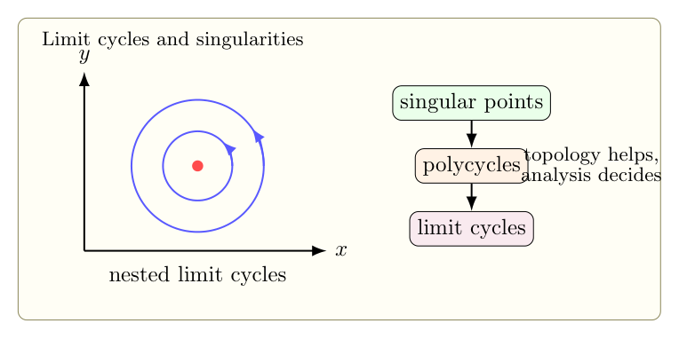
Try beginning with Bendixon-Poincaré theorem, which is classical stuff and belongs to a lot of textbooks on vector fields.
Affine invariance
The number of limit cycle is invariant under affine map.
Classification of singular point
Bezout theorem
Example
1..The graph is just like:
2..The graph is just like:
3..The graph is just like:
4..The graph is just like:
5..The graph is just like:
6.. The graph of it is just like:
Now we try to explain the phenomenon we see. At first we can see there is no limit cycle in the picture. The bifurcation place is just the place and is just like 3 lines. And there are two singularity .
7.
8.:
9.:
exist 2 limits cycles.
10.
Tree structure
In general, the lower bound of is established. first by Otrokov,and later proved to be .
If right, this upper bound estimate is combine of two things:
1.every limit cycle do not intersect.
2.every unclear limit cycle contain a singularity.
Rough strategy attack Hilbert 16th problem
Step1:
The first step is to do some simplify, we know the number of limit cycles do not change under a affine map , where A is a nonsingular 2*2 matrix. So we could classify the topological graph of the dynamic system.
Step2:
Classification the singularity under affine map, and investigate the topological graph of the topological graph of the singularity by floer cohomology. There is only finite type and we could focus on them one by one.
Every color in the graph is an area $P,Q$ do not have same component in it. And the boundary of areas is just the same component of if it exists.
Step3:
Bezout theorem tell us if two polynomials do not have same connected component then the intersection . And we can divide the space into finite parts, restrict to every part do not have the same component. And we have a upper bound control on the number of part when . A easy arrive bound could be .
Step4:
Now we focus ourself on 1 part where do not have same component on it. Now we begin to proof there will be a relationship between the limit cycle, very like a tree structure, it will combine with the following two thing:
Every limit cycle contains at least one singularity or one smaller limit cycle inside it.
2. Every pair of limit cycle , are limit cycle and is inside of , then there is at least one singularity or another limit cycle contain in .
This kind of topological result will lead to a upper bound of number of limit cycle and end the proof of Hilbert 16th problem.
Planar polynomial vector field for a harmonic pair of polynomials
In this case you can consider the heat equation . If the number of the limit cycle change, it must be the time to pass a singularity. and take , the dynamic system coverage to a very simlpe one and in particular it do not have limit cycle. So we need only look at the moments passing singularity.
Has the system of ODEs:
been studied for the special case of the polynomials and being a harmonic pair, i.e. the real and imaginary part of a holomorphic polynomial , ?
I am looking to learn a bit about (complex) ODEs and their interplay with algebraic geometry by some examples, but I couldn’t find anything on this special case in Ilyashenko’s survey on Hilbert 16 (I guess this case is too special and/or not very interesting as far as Hilbert 16 is concerned).
Nontheless, it seems very natural. If we set , this amounts to the equation $latex \int_{\gamma_t}\frac{dz}{F(z)}=t$
where is the curve “truncated” at and the RHS is in particular **real**. This can be taken further, for example by assuming is closed and using the residue theorem to obtain constraints on (the coefficients of) .
First, this case is totally uninteresting regarding Hilbert XVI. Indeed, there are no limit cycles in such systems. The -limit of a trajectory is either a point or a non-isolated cycle (center case).
A singularity at (*i.e.* a root of $F$) can only be of three types, according to the value of :
1. Source/focus: .
2. Center: .
3. Flower with petals: with multiplicity .
In addition there is a pole at infinity (if ) with exactly separatrices, reaching the singularity in finite time. The bassins of attraction / center regions attached to the above singularities are delimited by the separatrices.
[![enter image description here][2]][2]
S. Smale began to get interested in the question in the early 80’s while laying the foundations for BSS computational model (*The fundamental theorem of algebra and complexity theory*, 1981). He proposed a numerical root solver for polynomials by following the flow of . This started some works on the topic, for instance by Schub, Tischler, William (*The Newtonian graph of a complex polynomial*, 1988) or Benzinger (*Plane autonomous systems with rational vector fields*, 1991)…
In the case of these vector fields, the topological class is entirely encoded by their Newtonian graph (or the «dual» spinal graph) given by the incidence graph of the -limits of trajectories (in red on the picture). The main result for polynomials is that it is a tree. See *e.g.* Sverdlove (*Inverse problems for dynamical systems*,1981) and Schecter, Singer (*A class of vectorfields on $\mathbb S^2$ that are topologically equivalent to polynomial vectorfields*,1985) and Jongen, Jonker, Twilt (*On the classification of plane graphs representing structurally stable rational Newton flows*,1991).
The conformal classification has been initiated by Douady, Estrada and Sentenac (unpublished monograph, 2005) for the generic case (only focus/source singularities) and completed by Branner and Dias (*Classification of complex polynomial vector fields in one complex variable*, 2010). In addition to the combinatorial (topological) invariant, a complex «time-shift» (related to the integrals ) is associated to the separatrices, providing a complete conformal invariant.
In that latter context, the function is called a Fatou coordinates. It is a rectifying chart for the vector field, and has many interesting dynamical properties.
Notice also the deep and beautiful relationship between spinal graph and *Dessins d’enfants*, as established by Pilgrim (*Polynomial vector fields, dessins d’enfants, and circle packings*,2006), related to [this question](https://mathoverflow.net/questions/118527).
Classification of the singularity in even degree case.
Adjoint harmonic case have been studied. Look into the recent paper
Langley, J. K. Trajectories escaping to infinity in finite time. Proc. Amer. Math. Soc. 145 (2017), no. 5, 2107–2117, and the reference list in this paper.
They were also studied by physicists:
Bender, Carl M.; Hook, Daniel W.
Complex classical motion in potentials with poles and turning points.
Stud. Appl. Math. 133 (2014), no. 3, 318–336.
EDIT. I forgot to mention this:
B. Branner, K. Dias, Classification of complex polynomial vector fields in
one complex variable, Journal
Journal of Difference Equations and Applications
Volume 16, 2010 – Issue 5-6:
\section{Birkhoff回复定理蕴含Van Der Warden定理}
\subsection{Van Der Warden定理与它的动力系统解释}
这是一个组合定理,原始证明是很trick的,单遵老先生有一个证明,很trick,高中的时候尝试过证明,自己证了一个星期证明不出来就看掉了,现在回想起来应该跟当时的工具太原始了有关系。我想强调的是并不是数学思想的飞跃,而是数学工具的升级使得这个问题变简单了。\\
, is there a 2 order ordinary differential equation given by Sturm–Liouville theory such that the eigenfunction
is periodic if and only if
?
 , it does not mean
  .
. is a homomorphism then
 ).
). i.e.
i.e.  . Lifting to,
 .
. to
to  . (Regard
  as
as ![[0,2\pi]](https://s0.wp.com/latex.php?latex=%5B0%2C2%5Cpi%5D&bg=ffffff&fg=5e5e5e&s=0&c=20201002) ).
). . we get
  .
. and
and  in fact.
 is conjugate (in fact semi-conjugate is enough ). Then 1.If
 )
) ,
,  . It is not difficult to prove the rotation number of
  .
. we have that
  .
. . Then $latex\rho (T)$ is rational.
 has no periodic point then
  is irrational.
 .
.

 .
. .
. .
. ) and non-periodic pint (maybe orbits generated by
  .
. . Take any point
  , then:
 .
. .
. .
. .
. . $\forall x\in \mathbb S_1$ (if
  , take reflection
  ).
). such that
  . If not, we could prove rotation number is large than
  lead a contradiction.
 is a bounded monotonically increasing sequences in
  must satisfied
  .
. , and
, and  . If
. If  , then
  .
. between the set
  and
and  precise the natural ordering on
  .
. is a minimal orientation presenving homomorphism with irrational rotation number
  then
then  .
. . We define the variation of
  by:
by:

 has bounded variation if this value
  is finite.
 orientation preserving homomorphism of the circle with derivative of standard variation and irrational rotation number
  then
then  .
. and a sequences of integers
  such that the map:
  Then
Then  and write
  , for
, for  There exists an increasing sequences
  are all disjoint.
 because of existence of fix point.
 for
for  .
. always true for
  ?
? , but for what type of dynamic system
  . for all
  is not homomorphism but
  induced
  ,
,  is striating increasing, Is the limit of
  always exists? it could not be increase with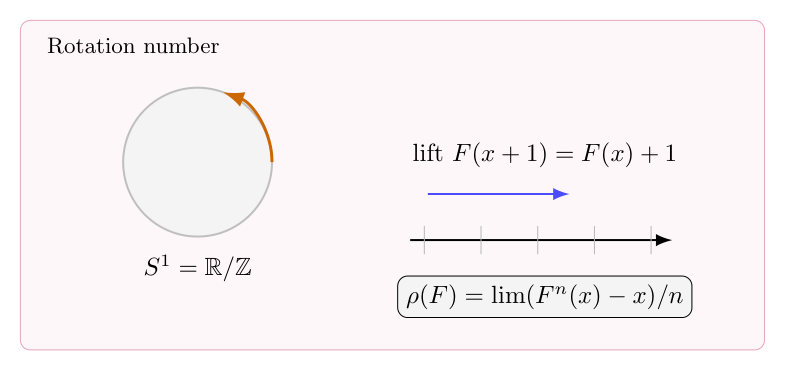

 is a given periodic matrix with period
  .
. .
. .
. . At least formally it could be solved:
 .
. is a multi-value function so
  , where
  is the identity matrix and
  is a solution of
 , it is equivalent to :
 , so is it true that for
  it do not have solution?
 case while
  could extend to
  and the identity
 . The key observation is
 ![log[(1+Y)(1+Y)]=log(1+X)+log(1+Y)](https://s0.wp.com/latex.php?latex=log%5B%281%2BY%29%281%2BY%29%5D%3Dlog%281%2BX%29%2Blog%281%2BY%29&bg=ffffff&fg=5e5e5e&s=0&c=20201002) always holds when
always holds when  , this will lead to a reasonable value of
![log[(1+X)(1+Y)]=log(1+X+Y+XY)](https://s0.wp.com/latex.php?latex=log%5B%281%2BX%29%281%2BY%29%5D%3Dlog%281%2BX%2BY%2BXY%29&bg=ffffff&fg=5e5e5e&s=0&c=20201002)
 and this process could be continue to the whole matrix space and the identity enjoy the accosted principle so
  is well-defined for all
  .
. for
for  is a continuous increasing function.
 as the quotient
  . Your homeomorphism
  lifts to a homeomorphism
 such that
  .
. , where
  is the composition
  times of
  with itself. By construction
  and
and  , so that
  factors as a homeomorphism of the circle conjugating
  too.
too.

 .
. ,
,  .
. is conjugate to the dynamic system
  , Not difficult to proof it is a homomorphism on
 be a entropy zero topological dynamic system. Let Mobius function be defined as
  , where $latex$ is the number of different primes occur in the decomposition of
  and
and  , observable
  is orthogonal to the Mobius function; i.e. ,
 is the skew product on
![[0,1]](https://s0.wp.com/latex.php?latex=%5B0%2C1%5D&bg=ffffff&fg=5e5e5e&s=0&c=20201002) .
. ,
, :
:
 , where
  .
.
 is suffice large primes pair.
 on
on  and the general case
  where A is a upper-triangle matrix with diagonal 1; i.e.
  , B is nilpotent. So the sarnak conjecture in this case is reduce to the Davenport estimate on exponent by B-Z-S theorem:
 ,
,  .
. , and it is easy to see there is only one case is nontrivial that is permutation:
  . We explain a little more with other trivial case:
 , the interval exchange map is just a rotation and for which the sarnak conjecture is just come from:
 ,
,  .
. .
. but it is a identity map on
  and the orbits of point only lying one of $I_1\cap I_2, I_3$, lying in which one depend on the original point
 which are not the common endpoint of them. Then you get two circle glue like a “8” , and
  is just rotate one of it and make the other one to be invariance.
 .
. , then
 ![A\cap B=\emptyset, A\cup B=[0,1]](https://s0.wp.com/latex.php?latex=A%5Ccap+B%3D%5Cemptyset%2C+A%5Ccup+B%3D%5B0%2C1%5D&bg=ffffff&fg=5e5e5e&s=0&c=20201002) . And
. And  ,
,  . the rotation
  ,
,  .
.
 , where
  is a
is a  invariant measure.

 varies in all sequences of measure coverage to
  in the sense for all
  ,
,  measurable then
  .
. , shift map on countable alphabet.
 diffeomorphisms on compact manifold is asymptotically h-expensive.
 metric space
 is a continuous map.
 , then
  is still a metric.
 . This identity could be proved by the cretition of entropy by
  -seperate set and
  .
. is the measure theoretic entropy of
  defined the moduli space of
  defined the moduli space of ergodic
  satisfied simplified entropy formula if
  surfaced small and
  ,
,  .
. .
. suffciently small,
  ,
,  .
. .
. .
.  ,
,  ,
,  , satisfied:
 weakly.
 ,
, 
 .
. be a compact riemannian manifold,
  is a diffeomorphism and
 is the multiplicity of
  and
and  .
. and
and  is equivalent to the Riemannian measure on
  diffemoephism, where
 is absolute continuous.
 have good regularity. But this idea is not complete to solve the problem.
 of
of  could be diagonal. Assume after diagonal the eigenvalue is
 .
. :
:
 ,
,  is the eigenvector space of
  . The dimension of $V_k$ is $dim V_k$.
 .
. , and we have:
 .
. . Estimate it is not very difficult. we need only observe the following two thing:
 exists a.e. in
  . and we product it and get :
 .
.


 .The graph is just like:
 .The graph is just like:


 .The graph is just like:
 .The graph is just like:
 .The graph is just like:
 . The graph of it is just like:
 and is just like 3 lines. And there are two singularity
  .
.


 :
:

 :
:


 is established. first
  by Otrokov,and later proved to be
  .
. , where A is a nonsingular 2*2 matrix. So we could classify the topological graph of the dynamic system.
 Every color in the graph is an area $P,Q$ do not have same component in it. And the boundary of areas is just the same component of
  if it exists.
 do not have same connected component then the intersection
  . And we can divide the space
  into finite parts,
  restrict to every part do not have the same component. And we have a upper bound control on the number of part when
  . A easy arrive bound could be
  .
. ,
,  are limit cycle and
  is inside of
  .
.
 . If the number of the limit cycle change, it must be the time to pass a singularity. and take
  , the dynamic system coverage to a very simlpe one and in particular it do not have limit cycle. So we need only look at the moments passing singularity.
 and
and  being a harmonic pair, i.e. the real and imaginary part of a holomorphic polynomial
  ,
,  ?
? , this amounts to the equation $latex \int_{\gamma_t}\frac{dz}{F(z)}=t$
 is the curve
  “truncated” at
  and the RHS is in particular **real**. This can be taken further, for example by assuming
  .
. -limit of a trajectory is either a point or a non-isolated cycle (center case).
 (*i.e.* a root of $F$) can only be of three types, according to the value of
  :
: .
. .
. petals:
  with multiplicity
  .
. ) with exactly
  separatrices, reaching the singularity in finite time. The bassins of attraction / center regions attached to the above singularities are delimited by the separatrices.
 . This started some works on the topic, for instance by Schub, Tischler, William (*The Newtonian graph of a complex polynomial*, 1988) or Benzinger (*Plane autonomous systems with rational vector fields*, 1991)…
 ) is associated to the separatrices, providing a complete conformal invariant.
 is called a Fatou coordinates. It is a rectifying chart for the vector field, and has many interesting dynamical properties.
 上的平移映射。
 的地方附近的环绕数计算,还有一些scalling变换或者是一些多尺度的问题里。\\
 open,
open, 或者
或者 开集,
开集, ,
, \\
\\ 是一个
是一个 集合
集合 这个集合是$T$不变的,第二点是注意到transitive point可以通过选取一组开集集进行描述从而有集合等式:
 所有的点都是transitivity point。\\
 不变的集合满足zorn lemma,所以有最小元\\
 分成若干个类,一定存在一个类存在任意长等差数列。\\
 装备上平移这个同胚构成的动力系统就够了,等差数列的存在性等价于若干个可以交换的映射,其实就是平移的步长不一样下的都回到原始值附近,这是birkhoff回复定理能够告诉我们的。\\
 在底空间上作用是transitive的,
 ,$T^iT^j=T^jT^i$,并不存在满足某种”一致”minimal的子空间。但是我们知道多重回复定理是对的。\\
 ,最后证明动力系统之间的半共轭会导致熵之间的不等式。
 情况的技巧
情况的技巧 这个会化简为简单的情况,再加上凸性。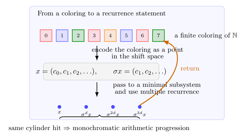
 中的可观测量是指
 ,$f\in C(T^2)$.
 ,由于
,由于 是
是 的一组基,只需对
 证明
证明 ,我们有\\
 \\
\\ \\
\\ \\
\\ \\
\\ \\
\\ :
:
 为多项式函数,我们有指数和估计:
 情形是引理的直接推论。接下来处理
 情形,这种情形下,我们定义
![\alpha=[q_1,q_2,q_3,....]](https://s0.wp.com/latex.php?latex=%5Calpha%3D%5Bq_1%2Cq_2%2Cq_3%2C....%5D&bg=ffffff&fg=5e5e5e&s=0&c=20201002)
 ,
, 那么:
那么:


 :\\定义
:\\定义 , 定义
, 定义 满足:\\
满足:\\ 的一段区间$I$,对任意
 ,
,

 \\
\\ 和
和 做cut off来简化问题。\\
 ,则
,则 .
. ,则根据分部积分公式
 .\\
.\\

 时,我们可以找到
 当$N\to \infty$,使得
 的部分可以被cut off.

![r_i \in [0,q_{i}-1]](https://s0.wp.com/latex.php?latex=r_i+%5Cin+%5B0%2Cq_%7Bi%7D-1%5D+&bg=ffffff&fg=5e5e5e&s=0&c=20201002)
 不为0,为什么要利用Ostrowoski表示,关键在于Ostrowoski表示中的标架
 是最佳逼近下最好的标架。\\
 标准长度
标准长度 如下:
如下:![l_1=\alpha,l_{k+1}=1-[\frac{1}{l_k}]l_k](https://s0.wp.com/latex.php?latex=l_1%3D%5Calpha%2Cl_%7Bk%2B1%7D%3D1-%5B%5Cfrac%7B1%7D%7Bl_k%7D%5Dl_k&bg=ffffff&fg=5e5e5e&s=0&c=20201002)
 ,做一些微小的计算会发现第k个

 在这个区间中的均匀分布性的余项可以得到很好地控制。
 ,对任意长度为
 的区间
的区间 ,
, 我们有:
我们有:
 提升为
提升为 ,因为实轴上长度为
 中的元素,有由于长度为
 的区间中有
的区间中有![[n\alpha]](https://s0.wp.com/latex.php?latex=%5Bn%5Calpha%5D&bg=ffffff&fg=5e5e5e&s=0&c=20201002) 个整数,所以:
个整数,所以:![\sum_{n=1}^N\chi_{(a,b)}(\{n\alpha\})=[N\alpha]=N(b-a)+O(1)](https://s0.wp.com/latex.php?latex=%5Csum_%7Bn%3D1%7D%5EN%5Cchi_%7B%28a%2Cb%29%7D%28%5C%7Bn%5Calpha%5C%7D%29%3D%5BN%5Calpha%5D%3DN%28b-a%29%2BO%281%29&bg=ffffff&fg=5e5e5e&s=0&c=20201002)