Hilbert 第十六问题笔记：limit cycle、奇点与拓扑图像

旧博客原文

原题：Hilbert 16th problem

Introduction

the statement of Hilbert’s 16th problem:

$H(n)<\infty?$

definition of $H(n)=max$

Limit cycle:

Try beginning with Bendixon-Poincaré theorem, which is classical stuff and belongs to a lot of textbooks on vector fields.

Affine invariance

The number of limit cycle is invariant under affine map.

Classification of singular point

Bezout theorem

Example

1. $\frac{dx}{dt}=y,\frac{dy}{dt}=x$ .The graph is just like:

2. $\frac{dx}{dt}=x^2+y^2,\frac{dy}{dt}=x-y$ .The graph is just like:

3. $\frac{dx}{dt}=x^2-y^2,\frac{dy}{dt}=5-y$ .The graph is just like:

4. $\frac{dx}{dt}=x^2-y^2,\frac{dy}{dt}=-y$ .The graph is just like:

5. $\frac{dx}{dt}=x^3-y^3,\frac{dy}{dt}=5-y$ .The graph is just like:

6. $\frac{dx}{dt}=y^2-x^2+1,\frac{dy}{dt}=y$ . The graph of it is just like:

7E54B6CB-B085-43F6-809C-918EAA380E9D

Now we try to explain the phenomenon we see. At first we can see there is no limit cycle in the picture. The bifurcation place is just the place $\frac{dx}{dt}=0\ or \frac{dy}{dt}=0$ and is just like 3 lines. And there are two singularity $(-1,0),(1,0)$ .

7. $\frac{dx}{dt}=y,\frac{dy}{dt}=y-x^2-x^2y$

0B2AEAFD-9FD7-491C-A28A-BB969E36AAB9

8. $\frac{dx}{dt}=y,\frac{dy}{dt}=y-x-x^2y$ :

9. $\frac{dx}{dt}=y(y-3),\frac{dy}{dt}=(y-3-x-x^2y)(y-x-x^2y)$ :

exist 2 limits cycles.

10. $\frac{dx}{dt}=y(y-3)(y-5),\frac{dy}{dt}(y-5-x-x^2y)(y-3-x-x^2y)(y-x-x^2y)$

Tree structure

In general, the lower bound of $H(n)$ is established. first $H(n)=O(n^2)$ by Otrokov,and later proved to be $H(x)=O(ln(n)n^2)$ .

If right, this upper bound estimate is combine of two things:

1.every limit cycle do not intersect.

2.every unclear limit cycle contain a singularity.

Rough strategy attack Hilbert 16th problem

Step1:

The first step is to do some simplify, we know the number of limit cycles do not change under a affine map $(x,y)\to (\hat x,\hat y)=(x,y)A$ , where A is a nonsingular 2*2 matrix. So we could classify the topological graph of the dynamic system.

Step2:

Classification the singularity under affine map, and investigate the topological graph of the topological graph of the singularity by floer cohomology. There is only finite type and we could focus on them one by one.

Every color in the graph is an area $P,Q$ do not have same component in it. And the boundary of areas is just the same component of $P,Q$ if it exists.

Step3:

Bezout theorem tell us if two polynomials $P(x,y), Q(x,y)$ do not have same connected component then the intersection $I_{P,Q}\leq deg(P)deg(Q)$ . And we can divide the space $R^2$ into finite parts, $P(x,y),Q(x,y)$ restrict to every part do not have the same component. And we have a upper bound control on the number of part when $\max\{deg(P(x,y)),deg(Q(x,y))\} \leq n$ . A easy arrive bound could be $4^n$ .

Step4:

Now we focus ourself on 1 part where $P(x,y),Q(x,y)$ do not have same component on it. Now we begin to proof there will be a relationship between the limit cycle, very like a tree structure, it will combine with the following two thing:

Every limit cycle contains at least one singularity or one smaller limit cycle inside it.

2. Every pair of limit cycle $(A,B)$ , $A,B$ are limit cycle and $A$ is inside of $B$ , then there is at least one singularity or another limit cycle contain in $\Omega$ .

This kind of topological result will lead to a upper bound of number of limit cycle and end the proof of Hilbert 16th problem.

Planar polynomial vector field for a harmonic pair of polynomials

In this case you can consider the heat equation $\partial_t u(z,t)=\Delta u(z,t)$ . If the number of the limit cycle change, it must be the time to pass a singularity. and take $t=\infty$ , the dynamic system coverage to a very simlpe one and in particular it do not have limit cycle. So we need only look at the moments passing singularity.

Has the system of ODEs:

$\frac{dx}{dt}=P(x,y)\\ \frac{dy}{dt}=Q(x,y)$

been studied for the special case of the polynomials $P$ and $Q$ being a harmonic pair, i.e. the real and imaginary part of a holomorphic polynomial $F=F(z)$ , $z=x+iy$ ?

I am looking to learn a bit about (complex) ODEs and their interplay with algebraic geometry by some examples, but I couldn’t find anything on this special case in Ilyashenko’s survey on Hilbert 16 (I guess this case is too special and/or not very interesting as far as Hilbert 16 is concerned).

Nontheless, it seems very natural. If we set $\gamma(t)=x(t)+iy(t)$ , this amounts to the equation $latex \int_{\gamma_t}\frac{dz}{F(z)}=t$
where $\gamma_t$ is the curve $\gamma$ “truncated” at $t$ and the RHS is in particular **real**. This can be taken further, for example by assuming $\gamma$ is closed and using the residue theorem to obtain constraints on (the coefficients of) $F$ .

First, this case is totally uninteresting regarding Hilbert XVI. Indeed, there are no limit cycles in such systems. The $\alpha / \omega$ -limit of a trajectory is either a point or a non-isolated cycle (center case).

A singularity at $a\in \mathbb C$ (*i.e.* a root of $F$) can only be of three types, according to the value of $F'(a)$ :

1. Source/focus: $F'(a)\notin i\mathbb R$ .
2. Center: $F'(a)\in i\mathbb R_{\neq 0}$ .
3. Flower with $2k$ petals: $F'(a)=0$ with multiplicity $k$ .

In addition there is a pole at infinity (if $\deg(F)>0$ ) with exactly $2\deg(F)$ separatrices, reaching the singularity in finite time. The bassins of attraction / center regions attached to the above singularities are delimited by the separatrices.

[![enter image description here][2]][2]

S. Smale began to get interested in the question in the early 80’s while laying the foundations for BSS computational model (*The fundamental theorem of algebra and complexity theory*, 1981). He proposed a numerical root solver for polynomials by following the flow of $\frac{F}{F'}$ . This started some works on the topic, for instance by Schub, Tischler, William (*The Newtonian graph of a complex polynomial*, 1988) or Benzinger (*Plane autonomous systems with rational vector fields*, 1991)…

In the case of these vector fields, the topological class is entirely encoded by their Newtonian graph (or the «dual» spinal graph) given by the incidence graph of the $\alpha / \omega$ -limits of trajectories (in red on the picture). The main result for polynomials is that it is a tree. See *e.g.* Sverdlove (*Inverse problems for dynamical systems*,1981) and Schecter, Singer (*A class of vectorfields on $\mathbb S^2$ that are topologically equivalent to polynomial vectorfields*,1985) and Jongen, Jonker, Twilt (*On the classification of plane graphs representing structurally stable rational Newton flows*,1991).

The conformal classification has been initiated by Douady, Estrada and Sentenac (unpublished monograph, 2005) for the generic case (only focus/source singularities) and completed by Branner and Dias (*Classification of complex polynomial vector fields in one complex variable*, 2010). In addition to the combinatorial (topological) invariant, a complex «time-shift» (related to the integrals $\int_\gamma\frac{1}{F(z)} dz$ ) is associated to the separatrices, providing a complete conformal invariant.

In that latter context, the function $\int\frac{1}{F(z)} dz$ is called a Fatou coordinates. It is a rectifying chart for the vector field, and has many interesting dynamical properties.

Notice also the deep and beautiful relationship between spinal graph and *Dessins d’enfants*, as established by Pilgrim (*Polynomial vector fields, dessins d’enfants, and circle packings*,2006), related to [this question](https://mathoverflow.net/questions/118527).

Reference

Classification of Singularities and Bifurcations of Critical Points of Even Functions

E.A.Kudryavtseva, E.Lakshtanov

Classification of the singularity in even degree case.

Adjoint harmonic case have been studied. Look into the recent paper
Langley, J. K. Trajectories escaping to infinity in finite time. Proc. Amer. Math. Soc. 145 (2017), no. 5, 2107–2117, and the reference list in this paper.

They were also studied by physicists:

Bender, Carl M.; Hook, Daniel W.
Complex classical motion in potentials with poles and turning points.
Stud. Appl. Math. 133 (2014), no. 3, 318–336.

EDIT. I forgot to mention this:

B. Branner, K. Dias, Classification of complex polynomial vector fields in
one complex variable, Journal
Journal of Difference Equations and Applications
Volume 16, 2010 – Issue 5-6:

补充说明

以下是新整理的中文说明；上方旧博客原文保持不变。

Hilbert 第十六问题的第二部分问：平面多项式向量场的 limit cycles 数量能否只用次数控制？这看起来像一个拓扑问题，因为 limit cycles 是平面轨道的闭曲线；但真正困难在于解析和代数几何结构如何控制这些闭轨道的产生与消失。

Hilbert 第十六问题笔记：limit cycle、奇点与拓扑图像 — Hilbert 第十六问题把 limit cycles、奇点、separatrix graph 和 return map 零点数放到同一个问题里。

1. 基本对象

考虑平面多项式系统

$$\dot x=P(x,y),\qquad \dot y=Q(x,y),$$

其中 $P,Q$ 是次数不超过 $d$ 的多项式。limit cycle 是孤立的周期轨道。Hilbert 第十六问题想问是否存在一个只依赖 $d$ 的上界 $H(d)$，控制所有这类系统的 limit cycles 数量。

对 $d=1$，线性系统没有孤立 limit cycles。对 $d\ge2$，问题迅速变得非常困难；一般情形至今仍未完全解决。

2. Poincare-Bendixson 的图像

Poincare-Bendixson theorem 告诉我们，平面系统的紧 $\omega$-limit set 若没有奇点，通常会落到周期轨道上。这使得二维动力系统比高维系统更有拓扑可视化：轨道、奇点、separatrices 和 limit cycles 共同组成一张平面图。

但可视化不等于容易。limit cycle 可以嵌套，可以从 polycycle bifurcation 中产生，也可能在参数变化时通过奇点附近的精细结构出现。

3. Affine invariance 与奇点分类

非退化 affine 变换不会改变 limit cycles 的数量。因此可以尝试先把系统化到较简单的坐标，再分类奇点局部模型。奇点由

$$P(x,y)=Q(x,y)=0$$

给出。若 $P,Q$ 没有公共因子，Bezout theorem 给出复射影意义下交点数不超过 $d^2$。这给了奇点数量的粗上界。

但是 limit cycles 不只由奇点数量决定。一个奇点周围可能有复杂的 separatrix structure；多个奇点之间的连接也可能产生 bifurcation。

4. 树结构的想法与局限

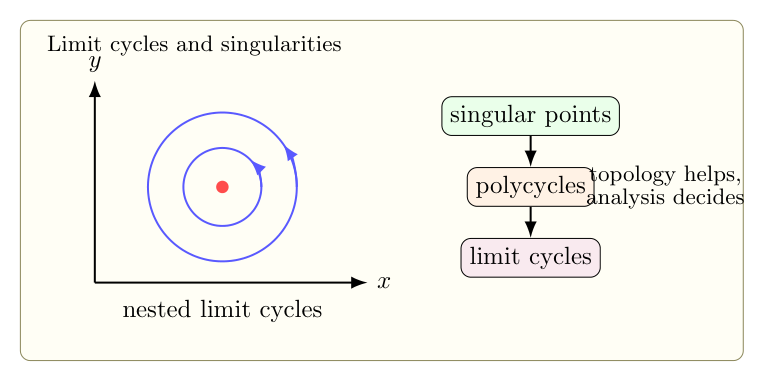
一个自然设想是把嵌套的 limit cycles 看成树：外层 cycle 包含内层 cycle 或奇点；两层之间的 annulus 里如果没有奇点，也许能排除新的孤立周期轨道。这样的拓扑图像确实有启发性。

困难在于，排除一个 annulus 中的周期轨道需要 Dulac function、Abelian integral、return map 或更精细的解析控制。拓扑结构给出框架，真正的上界需要估计 Poincare return map 的零点数。

5. Harmonic pair 的特殊情形

若 $P$ 和 $Q$ 是某个 holomorphic polynomial $F(z)$ 的实部和虚部，即

$$P+iQ=F(z),$$

则系统具有复分析结构。此时很多 Hilbert 第十六问题中的困难现象会消失：轨道可以通过

$$\int \frac{dz}{F(z)}=t$$

来理解，奇点由 $F$ 的零点控制。这样的系统通常不会给出 Hilbert XVI 中真正困难的孤立 limit cycles；它更像是一个用来学习复 ODE、Newtonian graph 和代数拓扑图像的模型。

6. 这条路线的意义

一个可能的攻击路线是：先用 affine 变换和 Bezout 控制奇点类型；再用 separatrix graph 把平面分解成有限区域；最后在每个区域中估计 return map 或 Dulac integral 的零点。这个策略很自然，但每一步都需要强解析输入。

Hilbert 第十六问题之所以难，正是因为它站在三件事的交界处：平面拓扑告诉我们轨道如何嵌套，代数几何控制多项式奇点，分析估计决定 limit cycles 能否真正出现。

Hilbert 第十六问题笔记：limit cycle、奇点与拓扑图像

旧博客原文

Planar polynomial vector field for a harmonic pair of polynomials

Reference

补充说明

1. 基本对象

2. Poincare-Bendixson 的图像

3. Affine invariance 与奇点分类

4. 树结构的想法与局限

5. Harmonic pair 的特殊情形

6. 这条路线的意义

评论

发表回复 取消回复

更多文章

从支撑接触到 Hausdorff 分层：凸 k-Hessian 解的四步证明机制

From Sum-Free Sets to Strongly 2-Primitive Sets: Localization, Patching, and the Search for Stability

[后端同步测试] 富媒体、代码与数学公式渲染

1

发表回复取消回复