这篇 note 介绍论文第3–6章的主证明。 目标是说明:若 $u$ 是开凸域 $\Omega$ 上满足
$$\sigma_k(D^2u)=1,\qquad 2\le k\le n,$$
的凸黏性解,则其非局部 $C^2$ 集满足
$$\mathcal H^{n-1}_{\mathrm{loc}}\bigl(\operatorname{Sing}(u)\bigr)=0.$$
证明把支撑接触集的维数、John 椭球的短轴、严格 section 的体积衰减和 Mooney 覆盖定理连接成一条闭合链。临界接触维数是 $q=n-k+1$。
This note introduces the main proof in Chapters 3–6. The goal is to explain why a convex viscosity solution $u$ on an open convex domain $\Omega$ satisfying
$$\sigma_k(D^2u)=1,\qquad 2\le k\le n,$$
has a non-locally-$C^2$ set obeying
$$\mathcal H^{n-1}_{\mathrm{loc}}\bigl(\operatorname{Sing}(u)\bigr)=0.$$
The proof joins the dimension of supporting contact sets, the short axes of John ellipsoids, volume decay of strict sections, and Mooney’s covering theorem into one closed chain. The critical contact dimension is $q=n-k+1$.
1. 接触分层与主证明链
对 $x\in\Omega$ 和 $p\in\partial u(x)$,令 $\ell_{x,p}$ 为相应的支撑仿射函数,并用 $d_u(x,p)$ 表示局部接触集 $\{u=\ell_{x,p}\}$ 在小尺度稳定后的仿射维数。定义
$$C_m(u)=\left\{x:d_u(x,p)\ge m\ \text{for every }p\in\partial u(x)\right\}.$$
“对每一个支撑斜率”是必要量词,因为第6章的 covering theorem 要求同一点的每一个 section 都满足体积衰减。
- 第3章:若某个支撑斜率的接触维数不超过 $n-k$,则 $u$ 在该点附近光滑。
- 第4章:正的 $k$-Hessian 密度控制小次水平集 John 椭球最短 $k$ 根轴的乘积。
- 第5章:$m$ 维接触与二次局部化共同产生 $|S_h|\lesssim h^{(m+k)/2}$。
- 第6章:Mooney 覆盖把 section 体积衰减转化为 Hausdorff 分层。
$$\operatorname{Sing}(u)\subset C_q(u),\qquad q=n-k+1,\qquad \mathcal H^{2n-m-k}_{\mathrm{loc}}\bigl(C_m(u)\bigr)=0.$$
最后取 $m=q$,便有 $2n-q-k=n-1$。
1. Contact strata and the proof chain
For $x\in\Omega$ and $p\in\partial u(x)$, let $\ell_{x,p}$ be the corresponding supporting affine function. Write $d_u(x,p)$ for the stabilized affine dimension, at small scales, of the local contact set $\{u=\ell_{x,p}\}$. Define
$$C_m(u)=\left\{x:d_u(x,p)\ge m\ \text{for every }p\in\partial u(x)\right\}.$$
The words “for every supporting slope” are essential because the covering theorem in Chapter 6 requires volume decay for every section at the point.
- Chapter 3: if one supporting slope has contact dimension at most $n-k$, then $u$ is smooth nearby.
- Chapter 4: positive $k$-Hessian density controls the product of the shortest $k$ axes of the John ellipsoid of a small sublevel set.
- Chapter 5: $m$-dimensional contact and quadratic localization together give $|S_h|\lesssim h^{(m+k)/2}$.
- Chapter 6: Mooney’s covering theorem converts section-volume decay into Hausdorff stratification.
$$\operatorname{Sing}(u)\subset C_q(u),\qquad q=n-k+1,\qquad \mathcal H^{2n-m-k}_{\mathrm{loc}}\bigl(C_m(u)\bigr)=0.$$
Taking $m=q$ gives $2n-q-k=n-1$.
2. 第一个引擎:小接触集推出局部光滑
这一节中,标准逼近、内点二阶估计和 Evans–Krylov 都是熟悉的步骤;真正决定论证能否启动的是一个马鞍面。减去一个支撑仿射函数后,归一化为 $u(0)=0$、$u\ge0$。若 $\{u=0\}$ 在小球内落入至多 $n-k$ 维的子空间 $Z$,取正交分解 $\mathbb R^n=Y\oplus Z$。此时 $\dim Y\ge k$;只需在 $Y$ 中选出 $k$ 个方向,并构造
$$Q(y,z)=A|y|^2-|z|^2+\alpha r^2.$$
这个马鞍面的两组方向承担相反而互补的任务:$Y$ 中至少 $k$ 个强正曲率方向保证 $D^2Q\in\Gamma_k$;沿接触空间 $Z$ 的负曲率则把 $Q$ 在球面边界压到 $u$ 的下方。选择 $A$、$\alpha$ 并适当缩放后,可以同时做到“边界上 $Q<u$”与“中心附近 $Q>u$”。这正是单纯凸抛物面无法提供的几何。
对 CNS 给出的光滑 $k$-admissible 逼近 $u_j$,选择正则值 $t_j$,并取包含原点的连通分支
$$D_j=\{Q-u_j>t_j\}.$$
边界与中心的符号差保证 $D_j$ 是困在小球内部的移动区域,而正则值保证其边界光滑。于是可以在 $D_j$ 上应用 Chou–Wang 局部二阶估计,得到与 $j$ 无关的 Hessian 界。随后对凹算子 $F=\sigma_k^{1/k}$ 使用 Evans–Krylov 与 Schauder,才得到极限 $u$ 的局部光滑性。
一致收敛 $u_j\to u$ 本身不产生 $C^2$ 极限;真正的正则化步骤是马鞍面切出的变化域和 Chou–Wang Hessian 界。
2. First engine: small contact sets imply local smoothness
The approximation, interior second-derivative estimate, and Evans–Krylov steps are standard; the device that actually starts the argument is a saddle surface. After subtracting a supporting affine function, normalize $u(0)=0$ and $u\ge0$. Suppose $\{u=0\}$ lies in a subspace $Z$ of dimension at most $n-k$ in a small ball. Split $\mathbb R^n=Y\oplus Z$. Then $\dim Y\ge k$; choose $k$ directions in $Y$ and construct
$$Q(y,z)=A|y|^2-|z|^2+\alpha r^2.$$
The two families of directions have opposite but complementary jobs. At least $k$ strongly positive curvatures in $Y$ ensure $D^2Q\in\Gamma_k$, while the negative curvature along the contact space $Z$ pushes $Q$ below $u$ on the spherical boundary. Choosing $A$ and $\alpha$, then scaling, gives both $Q<u$ on the boundary and $Q>u$ near the center. A purely convex paraboloid cannot provide this geometry.
For smooth $k$-admissible CNS approximations $u_j$, choose a regular value $t_j$ and take the component containing the origin of
$$D_j=\{Q-u_j>t_j\}.$$
The boundary/center sign change traps $D_j$ inside the small ball, and the regular value gives a smooth moving boundary. The localized Chou–Wang estimate then yields a Hessian bound independent of $j$ on $D_j$. Evans–Krylov for the concave operator $F=\sigma_k^{1/k}$, followed by Schauder estimates, yields local smoothness of the limit $u$.
Uniform convergence $u_j\to u$ does not by itself produce a $C^2$ limit. The genuine regularizing step is the moving domain cut out by the saddle surface together with the Chou–Wang Hessian estimate.
3. 第二个引擎:John 椭球与内部黏性测试
严格 section $K_h=\{u\le h\}\cap\overline B_R$ 虽然是凸集,却可能有复杂边界、随尺度旋转,并且各方向尺度相差很大;证明并没有假定它本身是椭球。John 定理的作用,是用一个内接椭球把这种高复杂度压缩成 $n$ 个半轴和一组主方向:
$$E_h=z_h+A_hB_1,\qquad E_h\subset K_h\subset z_h+nA_hB_1,$$
把 $A_h$ 的半轴按 $a_1\ge\cdots\ge a_n$ 排列。于是 section 的全部凸几何复杂度,在固定维数常数 $n$ 的损失内,变成了这 $n$ 根有序轴的账本。由 $E_h$ 构造测试函数
$$P_h(x)=h\left|A_h^{-1}(x-z_h)\right|^2.$$
令 $\mu_h=\min(P_h-u)$。平移后的 $P_h-\mu_h$ 在某个辅助内点 $y_h$ 从上方接触 $u$。因为 $D^2P_h=2hA_h^{-2}>0$,黏性不等式给出
$$a_q(h)\cdots a_n(h)\lesssim \lambda^{-1/2}h^{k/2},\qquad q=n-k+1.$$
这是最短 $k$ 根 John 轴乘积的上界。方程控制的是乘积,而不是每一根轴。
3. Second engine: John ellipsoids and an interior viscosity test
The strict section $K_h=\{u\le h\}\cap\overline B_R$ is convex, but its boundary may be complicated, its principal directions may rotate with scale, and its directional sizes may be wildly different. The proof does not assume that the section itself is an ellipsoid. John’s theorem compresses this geometric complexity into one inscribed ellipsoid, hence $n$ semiaxes and their principal directions:
$$E_h=z_h+A_hB_1,\qquad E_h\subset K_h\subset z_h+nA_hB_1,$$
Order the semiaxes of $A_h$ as $a_1\ge\cdots\ge a_n$. Up to the fixed dimensional factor $n$, the full convex-geometric complexity of the section has now become bookkeeping for these $n$ ordered axes. Construct the test function
$$P_h(x)=h\left|A_h^{-1}(x-z_h)\right|^2.$$
Set $\mu_h=\min(P_h-u)$. The translate $P_h-\mu_h$ touches $u$ from above at an auxiliary interior point $y_h$. Since $D^2P_h=2hA_h^{-2}>0$, the viscosity inequality gives
$$a_q(h)\cdots a_n(h)\lesssim \lambda^{-1/2}h^{k/2},\qquad q=n-k+1.$$
This is an upper bound for the product of the shortest $k$ John axes. The equation controls their product, not each axis separately.
4. 第三个引擎:接触维数与 section 体积
这一节的核心不是把 $K_h$ 想象成某个规则形状,而是把上一节得到的有序 John 轴分成三段。记 $q=n-k+1$。测试函数与黏性方程给出最短 $k$ 根轴的乘积上界
$$a_q\cdots a_n\lesssim \lambda^{-1/2}h^{k/2}.$$
另一方面,若支撑接触集含有半径 $\rho$ 的 $m$ 维相对球,John 上包含和宽度的极小极大表征给出 $a_m\gtrsim\rho$。由于 $a_1\ge\cdots\ge a_n$,这实际意味着
$$a_1,\ldots,a_m\gtrsim\rho.$$
当 $m\ge q$ 时,两段索引在中间确实重合:$a_q,\ldots,a_m$ 同时属于“接触给下界”的区间和“PDE 控制乘积”的区间。把这些已有下界的重合因子从短轴乘积中除去,便得到
$$a_{m+1}\cdots a_n\lesssim \lambda^{-1/2}\rho^{-(m-q+1)}h^{k/2}.$$
这一步迫使重合区间之后的最短 $n-m$ 根轴总体快速衰减,但还留下一个漏洞:前 $m$ 根轴虽然有下界,却完全可能非常长;所以仅靠上式还不能控制整个 section 的体积。修补这个漏洞的技巧是令
$$v(x)=u(x)+\frac{|x|^2}{2}.$$
加不加这个光滑二次函数,奇异集完全相同:$u$ 在一点附近属于 $C^2$ 当且仅当 $v$ 属于 $C^2$。这里也不对 $v$ 使用 $k$-Hessian 方程;所有 PDE 轴乘积估计仍来自 $u$。二次项只承担几何局部化。对相应严格 section,$v(x)\le h$ 立即蕴含 $|x|^2/2\le h$,因此
$$S_h^v\subset K_h\cap B_{\sqrt{2h}}.$$
这只是一项光滑抬升,却把可能任意长的前 $m$ 个接触方向全部截到 $O(\sqrt h)$,贡献 $h^{m/2}$;重合消去后剩余短轴的乘积贡献 $h^{k/2}$。两部分合在一起得到
$$|S_h^v|\lesssim \lambda^{-1/2}\rho^{-(m-q+1)}h^{(m+k)/2}.$$
4. Third engine: contact dimension and section volume
The point is not to imagine $K_h$ as a regular shape, but to split the ordered John axes from the previous section into three ranges. Put $q=n-k+1$. The test function and viscosity equation give the product bound for the shortest $k$ axes,
$$a_q\cdots a_n\lesssim \lambda^{-1/2}h^{k/2}.$$
On the other hand, if the supporting contact set contains a relative $m$-ball of radius $\rho$, the upper John inclusion and a width min-max argument give $a_m\gtrsim\rho$. Since $a_1\ge\cdots\ge a_n$, this means
$$a_1,\ldots,a_m\gtrsim\rho.$$
When $m\ge q$, the two index ranges genuinely overlap: $a_q,\ldots,a_m$ belong both to the contact-lower-bound range and to the PDE-controlled product. Dividing these overlap factors out of the short-axis product yields
$$a_{m+1}\cdots a_n\lesssim \lambda^{-1/2}\rho^{-(m-q+1)}h^{k/2}.$$
This forces rapid collective decay of the shortest $n-m$ axes after the overlap. A gap remains: the first $m$ axes have lower bounds but may still be arbitrarily long, so the last display alone does not control the volume of the whole section. The repair is to set
$$v(x)=u(x)+\frac{|x|^2}{2}.$$
Adding this smooth quadratic leaves the singular set unchanged: $u$ is locally $C^2$ at a point if and only if $v$ is. The $k$-Hessian equation is not applied to $v$; every PDE product estimate still comes from $u$. The quadratic term is used only for geometric localization. For the corresponding strict section, $v(x)\le h$ implies $|x|^2/2\le h$, hence
$$S_h^v\subset K_h\cap B_{\sqrt{2h}}.$$
This smooth lift truncates all potentially long first $m$ contact directions to $O(\sqrt h)$, contributing $h^{m/2}$; the remaining short-axis product after cancellation contributes $h^{k/2}$. Combining the two pieces gives
$$|S_h^v|\lesssim \lambda^{-1/2}\rho^{-(m-q+1)}h^{(m+k)/2}.$$
5. 第四个引擎:从体积衰减到 Hausdorff 分层
对 $x\in C_m(u)$ 以及 $v$ 的每一个支撑斜率,前一节给出
$$|S_h^v(x)|\le C_{x,p}h^{(m+k)/2}.$$
令 $s=m+k-n$,则 $(m+k)/2=(n+s)/2$。Mooney 的 section-covering theorem 因而推出
$$\mathcal H^{n-s}\bigl(C_m(u)\bigr)=\mathcal H^{2n-m-k}\bigl(C_m(u)\bigr)=0.$$
覆盖定理允许常数与高度阈值依赖 $(x,p)$,所以接触球半径 $\rho$ 没有统一下界并不妨碍论证。另一方面,满维接触会产生曲率任意小的上方二次测试,与 $\sigma_k\ge\lambda$ 矛盾,因此 $C_n(u)=\varnothing$。
第3章给出 $\operatorname{Sing}(u)\subset C_q(u)$。在 $m=q=n-k+1$ 处应用分层结论,便得到 $\mathcal H^{n-1}_{\mathrm{loc}}(\operatorname{Sing}(u))=0$。
5. Fourth engine: from volume decay to Hausdorff strata
For $x\in C_m(u)$ and every supporting slope of $v$, the previous section gives
$$|S_h^v(x)|\le C_{x,p}h^{(m+k)/2}.$$
Let $s=m+k-n$, so $(m+k)/2=(n+s)/2$. Mooney’s section-covering theorem yields
$$\mathcal H^{n-s}\bigl(C_m(u)\bigr)=\mathcal H^{2n-m-k}\bigl(C_m(u)\bigr)=0.$$
The covering theorem allows the constants and height thresholds to depend on $(x,p)$, so the absence of a uniform lower bound for the contact radius $\rho$ does not obstruct the argument. Full-dimensional contact, on the other hand, would produce an upper quadratic test of arbitrarily small curvature, contradicting $\sigma_k\ge\lambda$. Hence $C_n(u)=\varnothing$.
Chapter 3 gives $\operatorname{Sing}(u)\subset C_q(u)$. Applying the stratification result at $m=q=n-k+1$ yields $\mathcal H^{n-1}_{\mathrm{loc}}(\operatorname{Sing}(u))=0$.
6. 模型核算:$n=4$、$k=3$
此时 $q=2$。对临界层 $m=2$,接触几何给出 $a_2\gtrsim\rho$,而 PDE 给出 $a_2a_3a_4\lesssim h^{3/2}$。加入二次项后,
$$|S_h|\lesssim h^{5/2},\qquad \mathcal H^3(C_2)=0.$$
对更深的 $m=3$ 层,
$$|S_h|\lesssim h^3,\qquad \mathcal H^2(C_3)=0.$$
6. Model calculation: $n=4$, $k=3$
Here $q=2$. On the critical stratum $m=2$, contact geometry gives $a_2\gtrsim\rho$, while the PDE gives $a_2a_3a_4\lesssim h^{3/2}$. After adding the quadratic term,
$$|S_h|\lesssim h^{5/2},\qquad \mathcal H^3(C_2)=0.$$
For the deeper stratum $m=3$,
$$|S_h|\lesssim h^3,\qquad \mathcal H^2(C_3)=0.$$
7. 端点与限制
- $k=n$:$q=1$,结论恢复 Monge–Ampère 情形的 $\mathcal H^{n-m}(C_m)=0$。
- $k=2$:本方法给出临界接触层的余维一零测;全光滑还需要 strict $2$-convexity 的额外输入。
- 轴的控制:方程只控制短轴乘积,主轴可以随尺度旋转并重新分配,所以当前结论是 Hausdorff nullity,而不是统一 Minkowski packing。
7. Endpoints and limitations
- $k=n$: $q=1$ and the conclusion recovers the Monge–Ampère stratification $\mathcal H^{n-m}(C_m)=0$.
- $k=2$: this method gives codimension-one nullity for the critical contact stratum; full smoothness needs the additional input of strict $2$-convexity.
- Axis control: the equation controls only a product of short axes. Principal directions may rotate and redistribute with scale, so the conclusion is Hausdorff nullity rather than a uniform Minkowski packing estimate.
关于本文。 这是一篇介绍 Xiyu Hu, Sharp Hausdorff Bounds for the Interior Singular Set of Convex k-Hessian Solutions 第3–6章的证明导读 note。论文第8章的 mean-value 公式提供概念动机,但不作为上述主证明链的输入。
About this note. This is a proof-guide note to Chapters 3–6 of Xiyu Hu, Sharp Hausdorff Bounds for the Interior Singular Set of Convex k-Hessian Solutions. The mean-value formula in Chapter 8 provides conceptual motivation but is not an input to the proof chain above.
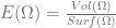
 , iff
, iff  is a ball,
  arrive a minimum .
 make the Energy
  arrive a minimum.


 , and let
  be a compact set. Let
  denote the [[Lebesgue measure]] (volume) of
  . Define the quantity
  by the ”’Minkowski–Steiner formula”’:

 , and:
 , so that:
 .
. -dimensional measure of the [[boundary (topology)|boundary]]
  of
of  ,
, are some [[continuous function]]s of
  (see [[quermassintegral]]s) and $\omega_{n}$ denotes the measure (volume) of the [[unit ball]] in
  :
: ,
, denotes the [[Gamma function]].
 gives the following well-known formula for the surface area of the [[sphere]] of radius
  ,
,  :
:
![= \lim_{\delta \to 0} \frac{[ (R + \delta)^{n} - R^{n} ] \omega_{n}}{\delta}](https://s0.wp.com/latex.php?latex=%3D+%5Clim_%7B%5Cdelta+%5Cto+0%7D+%5Cfrac%7B%5B+%28R+%2B+%5Cdelta%29%5E%7Bn%7D+-+R%5E%7Bn%7D+%5D+%5Comega_%7Bn%7D%7D%7B%5Cdelta%7D&bg=ffffff&fg=5e5e5e&s=0&c=20201002)
 ,
, is as above.
 .
. .
. with the Gromov-hausdorff metric on the space consist with convex open sets.
 points approximation in Gromov-hausdorff distance. and definitely carefully refinement of this kind of approximation could lead to the result of continuous of the energy
  it could be achieve with open convex set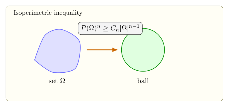
 estimate in the interior and