分类: PDE

  • 非线性椭圆方程平均值性质的几何直觉

    旧博客原文

    原题:Geometric intuition of mean value property of nonlinear elliptic equation

    I wish to gain some understanding of the MVP of nonlinear elliptic equation by geometric intuition.


    Linear elliptic equation case

    First of all, I have a very good geometric explain of the MVP of Laplace equation, i.e.

    MVP of laplace equation

    \Delta u=0 in \Omega , \forall B(x_0,r)\subset \Omega is a Ball, we have following identity:

    \frac{1}{\mu(\partial(B))}\int_{\partial B}u(x)dx=u(x_0)


    I need to point out first, this property is not difficult to proof by standard integral by part method, but the following method have more geometric intuition. And in some sense explain why this property holds.

    The proof is not very difficult to explain by mathematic formula, but I wish to divide the proof into two part, explain one part by graph and literal interpretation.

    part 1 of the proof:

    we consider a 1-parameter group of foliation, and consider the integral identity with this foliation.

    \int_{v\in S_{n-1}}\int_{\gamma_v} \frac{\partial \partial_{v}u}{\partial t}dt=\int_{B(x_0,r)}\partial_{n}u-\int_{S_{n-1}}\partial_{v}udv=\int_{B(x_0,r)}\partial_{n}u

    Part 2 of the proof:

    and we have:

      \int_{v\in S_{n-1}}\int_{\gamma_v} \frac{\partial \partial_{v}u}{\partial t}dt=0

    by the pointwise equation \Delta u=0, one key point is \partial_{-v-v}u=\partial_{vv}u, \forall v\in S_{n-1}.


    This approach cloud easily to transform to the general elliptic equation case and it seems a little difficult to transform to Possion equation, the non-hemomorphism case.


    Nonlinear elliptic equation case


    A-B-P estimate for general nonlinear uniformly elliptic equation


    ABP estimate is the most basic estimate in fully nonliear elliptic equation.
    The ABP maximum principle states (roughly) that, if

    a^{ij} \partial _i \partial _j u \geq f, in \ \Omega \subset \mathbb{R}^n (a^{ij} \geq C Id >0),

    Then (assuming sufficient regularity of the coefficients),

    \sup _{\Omega} u \leq \sup _{\partial \Omega} u + C (\int _{\Omega} \vert f \vert^n )^{1/n} ………. (*)

    I will give an intuitive explanation of the proof of (*) .
    Usually, in order to prove maximum principles, the key idea is to use that at a local max the second derivative is negative-definite, then choose a good basis and get some identity of 1-order drivative and inequality for 2-order’s. This process is used in such like the proof of the Hopf lemma, and some inter gradient estimate, consider some flexiable function like e^{Au} or sometihng else anyway.

    But in the proof of ABP we need more geometric intution and more trick.

    First we do a rescaling:
    if a^{ij} \partial _i \partial _j u \geq 1, in B_1 \subset \mathbb{R}^n (a^{ij} \geq C Id >0),u|_{\partial B_1}\geq 0.
    then:

    |inf_{B_1}u| \leq C |A|^{1/n} ....(**)

    And then We explain what is the contact set. It is the subset \Gamma^{+} of \Omega such that u agree with it convex envelop. i.e. \Gamma^{+}=\{x|u=convex \ evolap \ of \ u\ at \ x\} . The geometric meaning is it has at least one lower support plane. So what is \Gamma^{+} it is just the set that u is very low on it. Or in another way of view you consider -u as a lot of mountains then \Gamma^+ is the place near the tops of which mountain can see every thing (locally).
    Then we look at every point in \Gamma^{+} , then determination of the hessian matrix det(u_{ij}) at this point have a control due to the PDE a^{ij} \partial _i \partial _j u \geq 1, and the uniformly elliptic property.

    The determination of hessian matrix could be view as a determination of Jacobe matrix of the map (u_1,...,u_n)\to (e_1,...,e_n) .and by Area formula we have:

    \int_{\Phi(\Omega)}  f( \Phi^{-1}(y)) dy =\int_{\Omega}f(x)|J({\Phi(x)})| dx,

    It is easy to see for a constant c ,B_{c|sup_{\Omega}|u||}(0)\subset \Phi(\Omega) (Base on the PDE on every point, the geometric intution is just the function u could not be very narrow cone at every point). So we have , take f=\chi_{\Gamma^{+}} ,

    |B_{c\sup_{\Omega}|u|}(0)|^{n}\leq \int_{\Gamma^{+}}\chi_{\Gamma_{+}}(x)|J_{\Phi}(x)|dx

    so we have:

    |B_{c\sup_{\Omega}|u|}(0)|\lesssim |{\Gamma_{+}}|^{\frac{1}{n}}...(***)

    and the classical matrix inequality for every positive definite matrix A we have
    :

    det(AB)\leq (\frac{tr(AB)}{n})^n...(****) .

    combine (***),(****) ,we have:

    sup_{\Omega}|u|\lesssim ||\frac{a^{ij}u_{ij}}{D^*}||_{L^n({\Gamma^+})} .


    graph

    General approach to get MVP for elliptic equation which is come from geometry


    MVP for K-hessian equation, with geometric explanation


    MVP for K-curvature equation, with geometric explanation 


    MVP for p-Laplace equation, with geometric explanation


    补充说明

    以下是新整理的中文说明;上方旧博客原文保持不变。

    调和函数的平均值性质是椭圆方程最漂亮的几何现象之一。在线性情形,它来自球面对称和分部积分;在非线性椭圆方程中,真正的替代物往往不是严格平均值公式,而是 ABP estimate、contact set 和凸包几何。
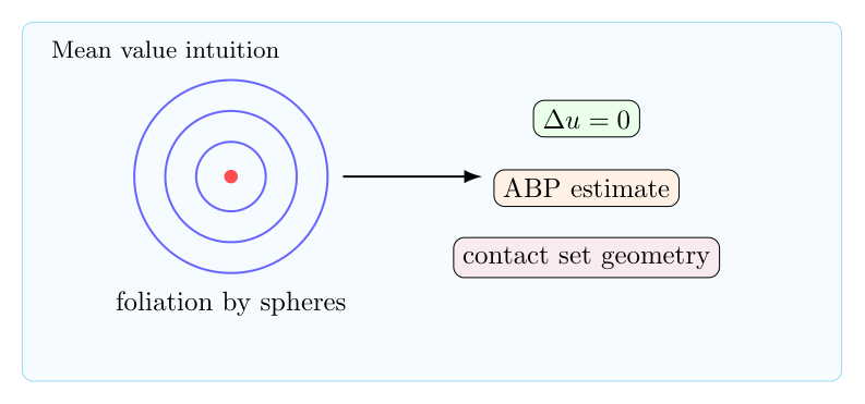
    非线性椭圆方程平均值性质的几何直觉
    线性调和函数有球面平均值性质,非线性椭圆方程则用 ABP estimate 和接触集合几何替代。

    1. Laplace 方程的平均值性质

    若 $\Delta u=0$,则对球 $B_r(x)$,

    $$u(x)=\frac1{|\partial B_r|}\int_{\partial B_r(x)}u\,d\sigma.$$

    证明可用 Green identity,也可以看成沿同心球 foliation 的通量守恒。

    2. 几何解释

    $$A(r)=\frac1{|\partial B_r|}\int_{\partial B_r(x)}u.$$

    对 $r$ 求导后,$\Delta u=0$ 让通量项消失,于是 $A(r)$ 为常数。球面对称和散度结构共同产生平均值性质。

    3. 非线性情形的问题

    对一般 fully nonlinear elliptic equation

    $$F(D^2u,x)=f,$$

    没有线性叠加,也没有简单的球面平均公式。我们需要用比较原理和接触几何替代平均值。

    4. ABP estimate

    ABP 最大值原理粗略地说给出

    $$\sup_\Omega u\le \sup_{\partial\Omega}u+C\|f\|_{L^n(\Omega)}.$$

    其证明看 $u$ 的凸包和 contact set。梯度映射的面积公式把函数的最大值和右端 $f$ 的积分联系起来。

    5. 一条直觉

    线性平均值性质说:每个点由周围平均决定。非线性椭圆理论说:最大值由接触集合和 Monge-Ampere 型几何控制。二者背后的共同点是椭圆性阻止信息沿单一方向集中,迫使解受到周围区域的整体约束。

  • Dirichlet 原理:从离散调和函数到连续调和函数

    旧博客原文

    原题:A discret to continuous approach to the Dirichlet principle.

    Direchlet principle:
    \Omega \subset R^n is a compact set with $C^1$ boundary. then there exists unique solution $f$ satisfied $\Delta f=0$ in $\Omega$, $f=g$ on \partial \Omega.

    Perron lifting and barrier function

    We know the standard approach of the Dirichlet principle is perron lifting and construction of barrier function on the boundary.

    The key point is if we define the variation energy E(u)=\int_{\Omega}|\nabla u|^2, then it is easy to see for u_1,u_2 is in perron set, E(sup (u_1,u_2))\geq \max\{E(u_1),E(u_2)\}. So we can begin from a maximization sequence to construct a Cauchy sequence by perron lifting and by the involve of barrier function to make the solution compatible with the boundary condition then arrive a proof.

    But when I was a freshman in undergraduate school and I do not know the method of perron lifting I try something I name it from discret to continuous approach to try to solved the problem. It is always a puzzle in my mind iff we can solve the Dirichlet principle in this way, roughly speaking, it is divid into two part:

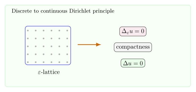
    1. Investigate the discretization of harmonic function in smaller and smaller scale. The discretization I consider is just \Omega\cap \epsilon \mathbb Z^2 i.e. the \epsilon-latties in $\Omega$,and discretization Laplace operator \Delta_{\epsilon}u(x_1,...,x_n)=\sum_{i_1,...,i_n\in\{-1,1\}}\frac{u(x_1+i_1,...,x_n+i_n)}{2^n}. Some result is much easier to arrive with the discretization thing, you know ,such as the existence of solution is just come from simple linear algebra. and we can deduce harneck inequality, gradient estimate, even green function. So we get a solution \hat f_{\epsilon} of \epsilon discretization and we do a extension \Omega\cap \epsilon \mathbb Z^2 to \Omega by take value of a small tube by the center of the tube, where the value have a definition by \hat f_{\epsilon}, and now we get f_{\epsilon}.


    2. The second step is to proof the solution f_{\epsilon} with \epsilon-discretization problem will coverage to the solution of original problem;i.e. we want to proof a L^{\infty} estimate;i.e. \forall \delta>0, \exists \epsilon>0, \forall 0<\epsilon_1,\epsilon_2<\epsilon we have \forall x\in \Omega, |f_{\epsilon_1}(x)-f_{\epsilon_2}(x)|<\delta. and by Albano-Ascoli theorem to construct f. Then we need to proof $f$ is the harmonic function we find, to verify this information we use the mean-value property. So we need to prove f satisfied mean-value property for every ball in \Omega.

    Here is my first question,
    > **Question 1:** How to prove the L^{\infty} estimate and the MVP of \epsilon-discretization will coverage to the MVP in R^n case occor in second step?

    My attempt to the L^{\infty} estimate is by renomelazation which seems could work, but the annoying thing is to proof the mean-value property will coverage to the real one, I try to use some result of random walk, but it seem not works…

    My second question is:
    > **Question 2:** Are this approach a universal phenomenon? At least could we use this approach to establish the existence of solution for linear elliptic and parabolic equation?

    The Third question is:
    > **Question 3:** If we consider some inverse problem, that is to say, form a MVP instead of a PDE to derive a solution, could this always be possible? some example is, if we change the mean value property for harmonic function from the average of ball to cube or triangle or elliptic or something else, what happen? Is there always a solution satisfied the news MVP point-wise? If not, Is there some counterexample? on another hand, if yes, are them came from some PDE?


    补充说明

    以下是新整理的中文说明;上方旧博客原文保持不变。

    Dirichlet 原理说:给定边界值,调和函数是 Dirichlet energy 的极小者。除了 Perron 方法和 barrier function,也可以从离散问题逼近连续问题。

    Dirichlet 原理:从离散调和函数到连续调和函数
    离散 Dirichlet 问题可由线性代数求解,再通过统一估计和紧性逼近连续调和函数。

    1. 连续问题

    设 $\Omega$ 有光滑边界,给定 $g$,要求

    $$\Delta u=0\quad\text{in }\Omega,\qquad u|_{\partial\Omega}=g.$$

    变分形式是极小化

    $$E(u)=\int_\Omega |\nabla u|^2\,dx.$$

    Euler-Lagrange 方程正是 Laplace 方程。

    2. 离散化

    取 $\varepsilon$-lattice 上的区域 $\Omega_\varepsilon$,定义离散 Laplacian

    $$\Delta_\varepsilon u(x)=\frac1{\varepsilon^2}\sum_{y\sim x}(u(y)-u(x)).$$

    离散 Dirichlet 问题是一个有限维线性代数问题,因此存在唯一解。

    3. 离散估计

    离散调和函数仍有最大值原理、Harnack inequality、Green function 和能量估计。这些估计若能与 $\varepsilon$ 无关,就可以取极限。

    4. 延拓与紧性

    把格点函数延拓为分片常数或分片线性函数。若能得到统一的 Holder 或 Sobolev 控制,就能通过 compactness 取出收敛子列。极限函数满足弱形式

    $$\int_\Omega \nabla u\cdot\nabla\varphi=0.$$

    5. 边界条件

    最细的是边界兼容性。Perron 方法中 barrier function 正是为处理边界极限;离散方法也需要离散 barrier,保证延拓后的极限真正取到给定边界值。

  • Gromov 式尺度思想在抛物方程中的应用

    旧博客原文

    原题:Gromov’s idea applicate to parabolic equation

    Gromov’s idea applicate to parabolic equation.

    Key point:

    1.rescaling+renormalization.

    2.analysis it on every scale.


    补充说明

    以下是新整理的中文说明;上方旧博客原文保持不变。

    抛物方程的一个基本特征是空间和时间的尺度不同:若空间尺度缩小为 $r$,时间尺度就应缩小为 $r^2$。Gromov 式思想强调:不要只在一个固定尺度看方程,而要不断 rescale、renormalize,并在每个尺度上寻找紧性和极限模型。

    Gromov 式尺度思想在抛物方程中的应用
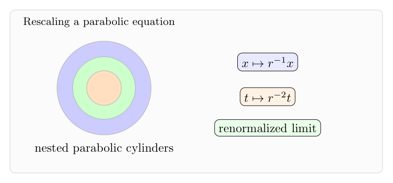
    抛物方程的自然尺度是空间 $r$、时间 $r^2$;正则性分析通常要在所有尺度上比较。

    1. 抛物缩放

    以热方程为例,若 $u_t-\Delta u=0$,定义

    $$u_r(x,t)=u(x_0+rx,t_0+r^2t).$$

    则 $u_r$ 仍满足同类方程。这个不变性说明,局部正则性问题可以被搬到单位尺度上处理。

    2. 重整化

    如果在某点附近梯度或曲率变大,就按最大量归一化。得到的序列若有紧性,极限通常是一个定义在全空间或半空间上的古老解。然后利用 Liouville theorem 排除非平凡极限。

    3. 每个尺度的分析

    尺度方法的关键不是一次缩放,而是在 dyadic scales 上反复比较:

    $$Q_r(z_0)=B_r(x_0)\times(t_0-r^2,t_0).$$

    若某个量在小尺度上不能衰减,就会产生 blow-up 极限;若 blow-up 极限被排除,就得到衰减估计。

    4. 与几何分析的联系

    Ricci flow、mean curvature flow 和非线性扩散方程中都可以看到这个结构。Gromov 风格的贡献在于把局部估计转成“所有尺度上的紧性与极限分类”。

  • k-Hessian 方程与 k-curvature 方程:椭圆性、测度与 Wolff 势

    旧博客原文

    原题:k-hessian equation and k-curvature equation

    here is the problem, how to understand k-hessian equation and k-curvature equation.

    k-hessian equation

    k-hessian equation is:

    H_k(u)=\sigma_k(D^2(u))=f (*)

    where u is admissible, i.e. \forall 1\leq i\leq k, \sigma_i(D^2(u))\geq 0. this is just the condition to make (*) be a elliptic equation.

    The most important result is the following three:

    1.sovable (*) with direchlet boundary condition.

    This is mainly the contribution of Caffaralli in 90’s. According flexible function and maximum principle we can establish the C^{1,\alpha} estimate and C^{2,\alpha} estimate in the inter. And the C^{2,\alpha} estimate near the boundary is establish according to the conformation invariant and some perbutation of the solution of k-hessian equation after special rescaling.

    2.Hessian measure.

    This is mainly the work of X.J.Wang and Trudinger. they proved:

    in the meaning of viscosity solution, if \sigma_k(D^2(u))=f. then we can associate a measure \mu with u,and the following is right:

    when u\in C^2(\Omega), \mu(B_r(x))=\int_{B_r{x}}\sigma_k(D^2(u)).

    if u_1,..,u_n,... coverage to u. then \mu_1,...,\mu_n,... coverage to \mu in weak sense.


    this is merely depend on a priori estimate on u

    3.pointwise estimate corresponding wolff potential.

    the Wolff potential is:

    W^{\mu}_{k}(x,r)= \int_{0}^r(\frac{\mu(B_t(x))}{t^{n-2k}})^{\frac{1}{k}}\frac{1}{t}dt

    We can easily use rescaling to understand the reasonable of this potential, and use this potential Lubutin establish the following pointwise estimate:

    u\in \Phi_k(B_{4R}(x)), u\leq 0, then we have:

    W^{\mu}_k(x,\frac{R}{2})\leq |u(0)| \leq W^{\mu}_k(x,2R)-sup_{B_{2R}}|u|


    the RHS could look as a corollary of classical A-B-P estimate. the LHS need combine several observation. mean-value property and some else.

    This result could use to establish some result on singularity point can be removable.

    k-curvature equation

    1.sovable (*) with direchlet boundary condition.

    This is also established by cafferalli.

    2.curvature measure.

    This is established very recently. mean curvature equation in 2014, by perron lift and modified, general case in 2016 by more complex calculate and method.

    3.pointwise estimate corresponding wolff potential.

    This still do not established, and is the main thing I focus on. Due to we can look as k-curvature as a “projection” of k-hessian equation, Calderon-Zegmund decomposition and the estimate of k-hessian equation maybe useful.


     My ideas

    look is as “average” of “loop space”, “surface space”.

    1.Grassmannian bundle

    n algebraic geometry, the Grassmann d-plane bundle of a vector bundle E on an algebraic scheme X is a scheme over X:
    {\displaystyle p:G_{d}(E)\to X}
    such that the fiber

    {\displaystyle p^{-1}(x)=G_{d}(E_{x})} is the Grassmannian of the d-dimensional vector subspaces of E_x. For example,

    {\displaystyle G_{1}(E)=\mathbb {P} (E)} is the projective bundle of E. In the other direction, a Grassmann bundle is a special case of a (partial) flag bundle. Concretely, the Grassmann bundle can be constructed as a Quot scheme.

    Like the usual Grassmannian, the Grassmann bundle comes with natural vector bundles on it; namely, there are universal or tautological subbundle S and universal quotient bundle Q that fit into

    {\displaystyle 0\to S\to p^{*}E\to Q\to 0}.
    Specifically, if V is in the fiber p−1(x), then the fiber of S over V is V itself; thus, S has rank r = rk(E) and

    {\displaystyle \wedge ^{r}S} is the determinant line bundle. Now, by the universal property of a projective bundle, the injection

    {\displaystyle \wedge ^{r}S\to p^{*}(\wedge ^{r}E)} corresponds to the morphism over X:
    {\displaystyle G_{d}(E)\to \mathbb {P} (\wedge ^{r}E)},
    which is nothing but a family of Plücker embeddings.

    The relative tangent bundle T Gd(E)/X of Gd(E) is given by[1]
    {\displaystyle T_{G_{d}(E)/X}=\operatorname {Hom} (S,Q)=S^{\vee }\otimes Q,}
    which is morally given by the second fundamental form. In particular, when d = 1, the early exact sequence tensored with the dual of S = O(-1) gives:
    {\displaystyle 0\to {\mathcal {O}}_{\mathbb {P} (E)}\to p^{*}E\otimes {\mathcal {O}}_{\mathbb {P} (E)}(1)\to T_{\mathbb {P} (E)/X}\to 0},
    which is the relative version of the Euler sequence.

    2.Explain of the fully nonlinear elliptic equation

    Now, we could consider the determination \sum_{i_1,...,i_k\in\{1,...,n\}}det(u_{ij})_{i,j\in \{i_1,...,i_k\}\times\{i_1,...,i_k\}} as the determination of transform: (u_{i_1},...,u_{i_k}) \longrightarrow (e_{i_1},...,e_{i_k}).

    Now we need to understand \sigma_k(D^2(u))=f at a point x_0 as the average of determination of transform matrix of (u_{i_1},...,u_{i_k}) \longrightarrow (e_{i_1},...,e_{i_k}) on Grassmannian manifold G_k(x_0) is equal to f(x_0), i.e.:

    \int_{G_k(x_0)} det(\frac{\partial u_{i_a}}{\partial e_{i_b}})     d\mu=f(x_0)

    where \mu is the natural haar measure on G_k(x_0) \simeq G_k.

    But the difficult to make the argument rigorous is that $u_i$ is scale and $e_i$ is vector.


    补充说明

    以下是新整理的中文说明;上方旧博客原文保持不变。

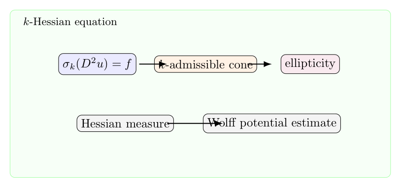
    $k$-Hessian 方程是完全非线性椭圆方程中的基本模型。它把 Hessian 矩阵特征值的第 $k$ 个基本对称函数作为主算子;椭圆性不再自动成立,而是依赖 admissible cone。

    k-Hessian 方程与 k-curvature 方程:椭圆性、测度与 Wolff 势
    $k$-Hessian 方程的椭圆性来自 admissible cone,弱解理论则进入 Hessian measure 和势估计。

    1. 方程与 admissibility

    设 $\lambda(D^2u)$ 是 Hessian 的特征值,定义

    $$S_k(D^2u)=\sigma_k(\lambda(D^2u)).$$

    $k$-Hessian 方程写作

    $$S_k(D^2u)=f.$$

    为了让方程椭圆,需要要求

    $$\lambda(D^2u)\in \Gamma_k=\{\sigma_1>0,\ldots,\sigma_k>0\}.$$

    这样的 $u$ 称为 $k$-admissible。这个条件是非线性椭圆理论的入口。

    2. Dirichlet 问题

    Dirichlet 问题要求

    $$S_k(D^2u)=f\quad\text{in }\Omega,\qquad u|_{\partial\Omega}=\varphi.$$

    经典策略是建立 $C^0$、梯度和二阶先验估计,再用连续性方法。边界估计通常最细,需要利用 domain 的几何条件、barrier function 和 rescaling。

    3. Hessian measure

    对非光滑 admissible 函数,也可以定义 Hessian measure。若 $u_j\to u$,并且 $u_j$ 是光滑 admissible,那么在合适条件下

    $$S_k(D^2u_j)\,dx \rightharpoonup \mu_k[u].$$

    这把方程扩展到 viscosity/pluripotential 风格的弱解框架。它类似 Monge-Ampere measure,但 $k$-Hessian 的 cone 结构更复杂。

    4. Wolff potential

    点态估计中会出现 Wolff potential:

    $$W_{\alpha,p}^\mu(x)=\int_0^\infty\left(\frac{\mu(B(x,r))}{r^{n-\alpha p}}\right)^{1/(p-1)}\frac{dr}{r}.$$

    它描述右端测度在不同尺度上的集中。对 $k$-Hessian 方程,解的上下界可以用相应的 Wolff potential 控制。这个形式可以从 scaling 看出:非线性阶数决定了势函数的指数。

    5. 与几何曲率方程的联系

    $k$-curvature 方程通常把 hypersurface 的第 $k$ 个曲率函数固定下来。解析上它和 Hessian 方程共享 symmetric polynomial、admissible cone 和 fully nonlinear ellipticity。几何问题中的正则性,往往依赖同一套先验估计和弱测度理论。

  • k-curvature 方程的正则性:连续性方法、屏障函数与边界估计

    旧博客原文

    原题:Regularity of k-curvature equation

    this is a note after reading the article”” of Cafferalli.

    in his article,a large type of fully nonlinear elliptic equation has been established.in particular,including the k-curvature equation.and use the continue method,we just need to establish a ingredient estimate,C^2 estimate in the interior and C^2 estimate near the boundary.we establish these estimate step by step,base on construct special flexible function and use the maximum principle to establish the first and second estimate,for the C^2 estimate near the boundary we need to investigate the influence of permutation on the boundary carefully.


    补充说明

    以下是新整理的中文说明;上方旧博客原文保持不变。

    $k$-curvature 方程属于完全非线性椭圆方程。典型形式可以写成

    $$F(D^2u,Du,u,x)=\sigma_k(\kappa[u])=\psi(x),$$

    其中 $\sigma_k$ 是主曲率的第 $k$ 个初等对称函数。Caffarelli-Nirenberg-Spruck 一类理论的核心是:在合适凸性锥中建立先验估计,然后用连续性方法得到解。

    k-curvature 方程的正则性:连续性方法、屏障函数与边界估计
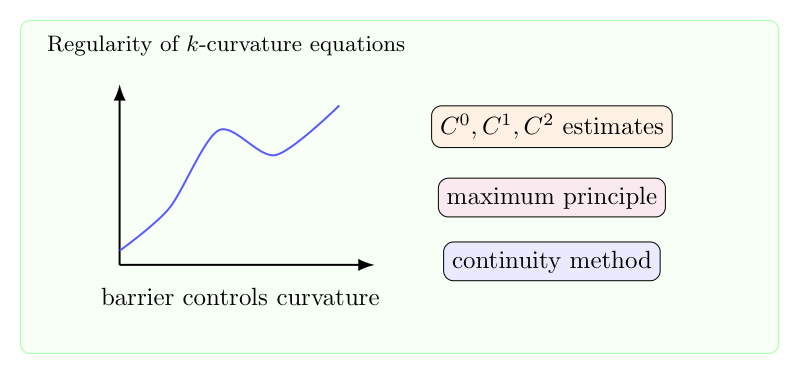
    k-curvature 方程的正则性证明依靠连续性方法、屏障函数、最大值原理和边界二阶估计。

    1. 连续性方法

    把目标方程嵌入一族方程 $F_t(u)=0$。若 $t=0$ 可解,开性来自线性化算子的可逆性,闭性则依赖统一先验估计。于是关键变成:

    $$\|u\|_{C^{2,\alpha}}\le C.$$

    2. 内部估计

    $C^0$ 和 $C^1$ 估计通常来自最大值原理与几何屏障。二阶估计更微妙,需要对最大特征值构造辅助函数,并利用方程的凹性抵消坏项。

    3. 边界估计

    边界附近最难的是混合二阶导数和法向二阶导数。这里要仔细利用边界曲率、可容许锥条件,以及对称函数 $\sigma_k$ 在坐标置换下的结构。

    4. 正则性升级

    一旦得到一致椭圆性和 $C^2$ 控制,可以通过 Evans-Krylov 定理得到 $C^{2,\alpha}$,再用 Schauder theory 提升到更高正则性。整个证明的脊梁是:屏障函数给低阶控制,最大值原理给二阶控制,椭圆正则性完成升级。

  • Heat flow 与多项式零点:从变形思想到 Riemann Hypothesis 的 toy model

    旧博客原文

    原题:Heat flow and the zero of polynomial-a approach to Riemann Hypesis

    this is a note after reading the blog:Heat flow and the zero of polynomial.

    1.instead of consider the original version:

    \partial_{zz}f(z,t)=\partial_tf(z,t).

    consider the corresponding “equidistribution version” is also interesting:

    \partial_{zz}f(z,t)=\theta(z,t)\partial_tf(z,t),especially \theta(z,t)=e^{2\pi i\alpha t},\alpha\in R-Q.

    2.

    where f(z)=z^n+a_{n-1}z^{n-1}+...+a_1z+a_0.

    f(z,t)=\sum_{k=1}^n\sum_{0\leq m\leq k-2,2|k-m}\frac{k!}{m!(k-m)!}z^mt^{k-m}.

    =\sum_{k=1}^m\sum_{0\leq m\leq k-2,2|k-m}C_k^mt^{k-m})z^mt^{k-m}

    \sum_{m=0}^{n-2}(\sum_{k=m,2|k-m}^nC_k^mt^{k-m})z^m.

    rescaling:

    F_t:(z_1(t),...,z_n(t))\longrightarrow (\frac{z_1(t)}{t},...,\frac{z_n(t)}{t}).

    F_t\cdot f(z,t)=\sum_{m=0}^{n-2}(\sum_{k=m,2|k-m}^nC_{k}^mt^{k-n})z^m.

    \lim_{t\to \infty}F_t\cdot f(z,t)=\sum_{m=0,2|n-m}^{n-2}C_n^mz^m.(*)

    even term \longrightarrow constant.(after renormelization)

    odd term \longrightarrow 0(invariant).so at least the sum zeros of is invarient.

    by the algebraic fundamental theorem,we have n zero \{z_1,...,z_n\}of (*).

    until now,we already now if the n zeros is distinct,then because the energy is the energy is the same and the entropy is increase so \exists T>>0,\forall t_i,t_j>T,\{t>T|z_i(t)\} \cap \{t>T|z_j(t)\}=\emptyset.\lim_{t\to \infty}|z_i(t)|=\infty and \lim_{t\to \infty}arg(z_i(t))=z_i.

    but how to know the information of the change of direction at “blow up” time?

    1.change direction only at blow up.

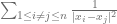
    2.energy invariant \sum_{1\leq i\neq j\leq n}\frac{1}{|x_i-x_j|^2}.

    3.general philosophy

    deformation some function under some evolution equation, such like heat equation,wave equation,shrodinger equation.and there is some conversion thing under the equation,and some quantity that could calculate directly such like the trace of spectral.

    4.difficultis

    this philosophy could generate to the analytic function case,but to make the limit case(I only know how ti deal with this now)coverage.we need very good control on the coefficient.

    and to investigate the change of direction at blow up point maybe we need some knowledge about the burid group.


    补充说明

    以下是新整理的中文说明;上方旧博客原文保持不变。

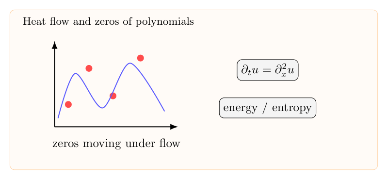
    用 heat flow 研究多项式零点,是理解更复杂解析函数零点问题的一个 toy model。基本思想是:让函数随时间演化,观察零点如何移动,以及哪些量在演化中保持或单调。

    Heat flow 与多项式零点:从变形思想到 Riemann Hypothesis 的 toy model
    heat flow 让多项式零点随时间运动,提供研究零点实性和不变量的 toy model。

    1. 多项式的 heat deformation

    设 $P(x)$ 是多项式,考虑

    $$\partial_t u=\partial_x^2u,\qquad u(0,x)=P(x).$$

    因为 heat operator 保持多项式空间,$u(t,x)$ 仍然是多项式。其零点随 $t$ 移动。

    2. 不变量与单调量

    某些系数组合在演化中保持不变,另一些量具有单调性。例如最高次项不变,低阶偶次项会随 heat flow 改变。零点的质心或某些对称量可能保持。

    3. 零点碰撞

    若零点始终实且互异,运动图像较清楚;真正困难发生在零点碰撞或分裂时。此时需要理解 blow-up 时间附近的方向变化。

    4. 与 Riemann Hypothesis 的类比

    de Bruijn-Newman 常数研究的是 Xi 函数在 heat flow 型变形下零点保持实的临界时间。多项式模型不能证明 RH,但能展示同一种哲学:通过演化方程追踪零点几何。

    5. 需要的估计

    要从多项式推广到整函数,必须控制系数、增长阶和极限过程。多项式情形的代数基本定理给出有限零点;整函数情形需要更强的紧性和零点分布估计。

  • Schauder estimate 与 Sobolev inequality:椭圆方程正则性的两种语言

    旧博客原文

    原题:Schauder estimate and Sobelov inequality

    In this note we discuss the Schauder theory for uniformly elliptic linear equations and Sobelov inequality.

    the three main topics ars a priori estimate in Holder norms,regularity of arbitrary solutions and the solvability of the Dirichlet problem.Among these topics,a priori estimates are the most fundamental and the basis of the follows two.we will discuss both the interior Schauder estimate and global Schauder estimate.

    -Schauder Theory-

    1. Interior Schauder Theory

    {\Omega} be a domain in {R^n},bounded most of the time.
    {a_{ij},b_i,c} be defined in {\Omega},with {a_{ij}=a_{ji}}.where {1\leq i,j\leq n}.
    we consider the operator {L} given by,

    \displaystyle Lu=a_{ij}\partial_{ij}u+b_i\partial_iu+c,in \ \Omega.

    easy to see {Lu} is defined for any {u\in C^2(\Omega)}.
    the operator {L} is always be assumed to be strictly elliptic in {\Omega};namely,
    \displaystyle a{ij}\xi_i\xi_j \geq \lambda|\xi|^2

    for any {\xi\in R^n,x\in \Omega},where {\lambda} is a positive constant.
    1.1. Interior Schauder Estimate

    define the weighted {C^{k,\alpha}} norm,

    \displaystyle |u|^*_{C^{k,\alpha}(B_R)}=\sum_{i=0}^k R^i|D^iu|_{L^{\infty}(B_R)}+R^{k+\alpha}[D^ku]_{C^{\alpha}(B_R)}

    easy to see {R} come from a scaling.
    consider the PDE.
    \displaystyle Lu=a_{ij}\partial_{ij}u+b_i\partial_iu+c=f,in \ \Omega.

    we want to proof this type estimate,
    \displaystyle |u|_{C^{2,\alpha}(A)} \leq C(|u|_{L^{\infty}(\Omega)}+|f|_{C^{\alpha}(\Omega)})

    where {A\subset \Omega }
    we first deal with a easy case,{a_{ij}} is constant. in this case we proof the estimate:

    Lemma 1 {f \in C^{\alpha}(B_R)},for some {\alpha \in (0,1)},and {(a_{ij})} be a constant symmetric {n\times n} matrix satisfying
    \displaystyle \lambda |\xi|^2 \leq a_{ij}\xi_i\xi_j \leq \Lambda|\xi|^2

    {\exists \lambda,\Lambda >0,\forall \xi \in R^n}. suppose {u\in C^2(B_R)} satisfies:
    \displaystyle a_{ij}\partial_{ij}u=f, in \ B_R

    then ,{u \in C^{2,\alpha}(B_{\frac{R}{2}})},moreover,
    \displaystyle |u|^*_{C^{2,\alpha}(B_{\frac{R}{2}})}\leq C[|u|_{L^{\infty}(B_R)}+R^2|f|^*_{C^{\alpha}(B_R)}]

    Proof: \Box to continue,we prove an interpolation inequality for Holder continuous functions.

    Lemma 2 Let {\alpha,\mu \in (0,1)} and {B_R} be a ball of radius {R} in {R^n},then, (1)for any {u\in C^{1,\alpha}(\overline B_R)},
    \displaystyle \mu^{\alpha}R^{\alpha}[u]_{C^{\alpha}(B_R)}\leq C[\mu R |\nabla u|_{L^{\infty}(B_R)}+|u|_{L^{\infty}(B_1)}]

    (2)for any {u\in C^{1,\alpha}(\overline B_R)},
    \displaystyle \mu R |\nabla u|_{L^{\infty}(B_R)} \leq C[\mu^{1+\alpha}R^{1+\alpha}|\nabla u|_{C^{\alpha}(B_R)}+|u|_{L^{\infty}(B_1)}]

    (3)for any {u\in C^2(\overline B_R)},
    \displaystyle \mu R|\nabla u|_{L^{\infty}(B_R)}\leq C[\mu^2R^2|\nabla^2 u|_{L^{\infty}(B_R)}+|u|_{L^{\infty}(B_R)}]

    where {C} is a positive constant depending on n and {\alpha}.
    Proof: \Box

    Corollary 3 Let {\alpha,\mu\in (0,1)} and {B_R} be a ball of radius {R} in {R^n}.Then,for any {u\in C^{2,\alpha}(\overline B_R)},
    \displaystyle \sum_{i=0}^2(\mu R)^i|\nabla^i u|_{L^{\infty}(B_R)}+\sum_{i=0}^1(\mu R)^{i+\alpha}[\nabla^i u]_{C^{\alpha}(B_R)}\leq C[(\mu R)^{2+\alpha}[\nabla^2 u]_{C^{\alpha}(B_R)}+|u|_{L^{\infty}(B_R)}]

    Proof: \Box

    Now we are ready to prove an interior estimate for {C^{2,\alpha}}-norms of solutions of uniformly elliptic equations.The trick is to freeze coefficients.

    Lemma 4
    2. Global Schauder Theory


    -Sobelov inequality-

    Theorem 5
    \displaystyle W_0^{1,p}(\Omega)\longrightarrow L^{\frac{np}{n-p}}(\Omega),1\leq p <n

    moreover,we have: {\exists C=C(n,p)}, {\forall u\in W^{1,p}_0(\Omega)},
    \displaystyle ||u||_{\frac{np}{n-p}} \leq C||Du||_p,1\leq p<n

    Proof:

    \displaystyle p=1

    suffice to proof:
    \displaystyle ||u||_{\frac{n}{n-1}}\leq C||Du||_1

    obvious we have:
    \displaystyle |u(x)|\leq \int_{-\infty}^{\infty}|Du(x)|dx

    so {\int_{\Omega} |u|^{\frac{n}{n-1}}\leq \int_{\Omega} \Pi_{i=1}^n(\int_{-\infty}^{\infty}|D_iu(x)|dx)^{\frac{1}{n-1}}}.
    so {||u||_{\frac{n}{n-1}}\leq (\int_{\Omega}\Pi_{i=1}^n(\int_{-\infty}^{\infty}|D_iu|)^{\frac{1}{n-1}})^{\frac{n-1}{n}}\leq \int_{\Omega} \Pi_{i=1}^n(\int_{-\infty}^{\infty}|D_iu|)^{\frac{1}{n}} \leq \int_{\Omega} \frac{1}{n} \sum_{i=1}^n(\int_{-\infty}^{\infty}|D_iu|)\leq C||Du||_1}
    \displaystyle 1<p<n

    use the similar argument as {p=1} to prove the situation {1<p<n}.
    suffice to prove {||u||_{\frac{np}{n-p}}\leq C||Du||_p}.
    obvious we have:{|u(x)|^p\leq \int_{-\infty}^{\infty}p|u|^{p-1}|Du|}.
    {(\int_{\Omega}|u(x)|^{\frac{np}{n-p}})^{\frac{n-p}{np}}}
    {\leq (\int_{\Omega} \Pi_{i=1}(\int_{-\infty}^{\infty} p|u|^{p-1}|D_iu| )^{\frac{1}{n-p}})^{\frac{n-p}{np}} }
    {\leq C\int_{\Omega} \Pi_{i=1}^n(\int_{-\infty}^{\infty}p|u|^{p-1}|D_iu|)^{\frac{1}{np}}}
    {\leq\frac{c}{n}\sum_{i=1}^n\int_{\Omega}(\int_{-\infty}^{\infty}p|u|^{p-1}|D_iu|)^{\frac{1}{p}}}
    {\leq \frac{c}{n}\sum_{i=1}^n\tilde C p[(\int_{\Omega} (|u|^{p-1})^{\frac{p}{p-1}})^{\frac{p-1}{p}}+(\int_{\Omega} |D_iu|^p)^{\frac{1}{p}}]^{\frac{1}{p}} }
    {\leq C||Du||_p}. Q.E.D. \Box
    4.

    \displaystyle W_0^{1,p}(\Omega)\longrightarrow C(\bar\Omega),n<p

    moreover,we have: {\exists C=C(n,p)}, {\forall u\in W^{1,p}_0(\Omega)},
    \displaystyle sup_{\Omega}|u| \leq C|\Omega|^{\frac{1}{n}-\frac{1}{p}}||Du||_p,p>n

    {\mu\in (0,1]},

    \displaystyle (V_{\mu}f)(x)=\int_{\Omega}|x-y|^{n(\mu-1)}f(y)dy

    then {V_{\mu}: L^1(\Omega) \longrightarrow L^1(\Omega) } is well-defined by the following lemma:
    Lemma 6 {V_{\mu}:L^p \longrightarrow L^q} continously for any q,{1\leq q \leq \infty} satisfy {0\leq \delta=\delta(p,q)=\frac{1}{p}-\frac{1}{q} \leq \mu}.
    furthermore,for any {f\in L^p(\Omega)}
    \displaystyle ||V_{\mu}f||_q \leq (\frac{1-\delta}{\mu -\delta})^{1-\delta}w_n^{1-\mu}|\Omega|^{\mu-\delta}||f||_p

    Proof: {h(x-y)=|x-y|^n(\mu-1)} directly calculate follows that :

    \displaystyle ||h||_r \leq (\frac{1-\delta}{\mu -\delta})^{1-\delta} w_n^{1-\mu}|\Omega|^{\mu-\delta}

    now follows young inequality and this priori estimate we have:
    {||V_{\mu}f||_q=(\int_{\Omega}(\int_{\Omega}|x-y|^{n(\mu-1)}f(y)dy)dx)^{\frac{1}{q}}}
    {\leq (\int_{\Omega}(\int_{\Omega}h^{\frac{r}{q}}h^{r(1-\frac{1}{p})}|f|^{\frac{p}{q}}|f|^{p\delta})^qdx)^{\frac{1}{q}}}
    {\leq (\int_{\Omega}(\int (h^r|f|^p)^{\frac{1}{q}}(\int h^r)^{1-\frac{1}{p}}(\int f^p)^{\delta})^{q})^{\frac{1}{q}}}
    {\Longrightarrow}
    \displaystyle ||V_{\mu}f||_q \leq sup_{x \in \Omega} \{\int h^r(x-y)dy\}^{\frac{1}{r}}||f||_p

    and by the priori estimate,we have:
    \displaystyle ||V_{\mu}f||_q \leq (\frac{1-\delta}{\mu -\delta})^{1-\delta}w_n^{1-\mu}|\Omega|^{\mu-\delta}||f||_p

    Q.E.D. \Box
    Lemma 7 {f\in L^p(\Omega)},{g=V_{\mu}f}.
    {\Longrightarrow} {\exists c_1,c_2} constant depend only on {n,p},such that
    \displaystyle \int_{\Omega} exp[\frac{g}{c_1||f||_p}]^{p^`}dx\leq c_2|\Omega|,p^`=\frac{p}{p-1}

    Proof: we have

    \displaystyle ||g||_q \leq q^{1-\frac{1}{p}+\frac{1}{q}}w_n^{1-\frac{1}{p}}|\Omega|^{\frac{1}{q}}||f||_p

    {\Longrightarrow}
    \displaystyle \int_{\Omega} |g|^{p^`q}dx \leq p^`q(w_np^`q||f||_p^{p^`})^q|\Omega|

    {\Longrightarrow}
    \displaystyle \int_{\Omega}\sum_{N_0}^{N}\frac{1}{k!}(\frac{|g|}{c_1||f||_p})^{p^`k}\leq p^`|\Omega|\sum(\frac{p^`w_n}{c_1^p})^k\frac{k^k}{(k-1)!}

    then take {c_1,c_2} suffice large. Q.E.D. \Box
    Lemma 8 let {u\in W^{1,1}_0(\Omega)}
    \displaystyle u(x)=\frac{1}{nw_n} \int_{\Omega} \frac{(x_i-y_i)D_iu(y)}{|x-y|^n}

    a.e. in {\Omega}.
    Proof: frist zero extended {u} to whole space.and we have {u(x)=\int_{-\infty}^xD_iu(x)}.

    \displaystyle u(x)=\int_0^{\infty}D_ru(x+rw)dr

    forall {w\in \partial B_1(0)},so
    \displaystyle u(x)=-\frac{1}{nw_n}\int_0^{\infty}\int_{|w|=1}D_ru(x+rw)drdw=\frac{1}{nw_n}\int_{\Omega}\frac{(x_i-y_i)D_iu(y))}{|x-y|^ndy}

    Q.E.D. \Box
    Theorem 9 let {u\in W^{1,n}_0(\Omega)},then there exists constant {c_1,c_2} such that
    \displaystyle \int_{\Omega}exp[\frac{|u|}{c_1||Du||_n}]^{\frac{n}{n-1}}dx\leq c_2|\Omega|

    Proof: a \Box

    Theorem 10 {u\in W_0^{1,p}(\Omega),p>n},then {u\in C^{\gamma}(\Omega)},{\gamma=1-\frac{n}{p}}.
    moreover {\forall ball B=B_R}
    \displaystyle osc_{\Omega \cap B_R}u \leq C R^{\gamma} ||Du||_p

    Proof: a \Box


    补充说明

    以下是新整理的中文说明;上方旧博客原文保持不变。

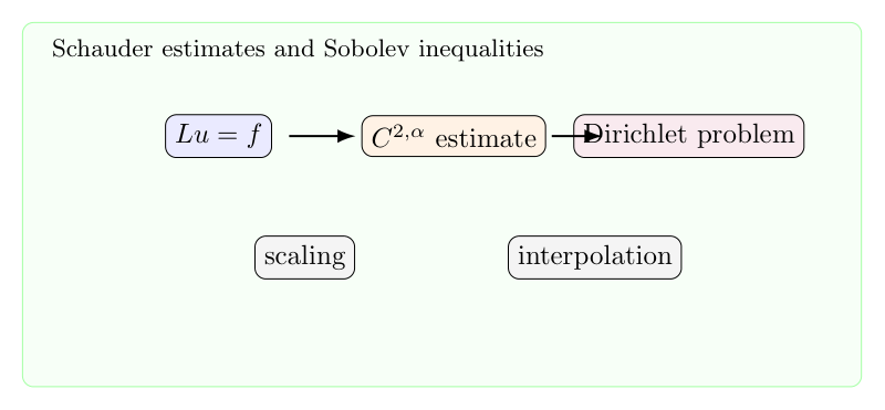
    Schauder 理论和 Sobolev 理论是椭圆方程正则性的两套基本语言。前者追踪 Holder 范数,适合系数和右端足够连续的情形;后者追踪积分可积性,适合弱解和变分方法。

    Schauder estimate 与 Sobolev inequality:椭圆方程正则性的两种语言
    Schauder 估计追踪 Holder 正则性,Sobolev 不等式追踪积分正则性,两者共同构成椭圆方程的基本正则性工具。

    1. 线性一致椭圆算子

    考虑

    $$Lu=a^{ij}(x)\partial_{ij}u+b^i(x)\partial_i u+c(x)u=f.$$

    一致椭圆性是指存在 $\lambda>0$,使

    $$a^{ij}(x)\xi_i\xi_j\ge \lambda|\xi|^2.$$

    这是所有先验估计的起点。

    2. Interior Schauder estimate

    若系数和 $f$ 都在 $C^\alpha$ 中,则局部有

    $$\|u\|_{C^{2,\alpha}(B_{1/2})}\le C\bigl(\|u\|_{C^0(B_1)}+\|f\|_{C^\alpha(B_1)}\bigr).$$

    常系数情形可以先通过 Newton potential 或 Fourier 方法得到,再用冻结系数和 perturbation 推广到变系数情形。

    3. Scaling 与 weighted norms

    Schauder 估计的形状由 scaling 决定。若把球 $B_r$ 缩放到单位球,二阶导数带来 $r^{-2}$,Holder seminorm 还会多出 $r^{-\alpha}$。weighted norm 正是为了把这些尺度因子记录清楚。

    4. Sobolev inequality

    Sobolev 不等式给出

    $$\|u\|_{L^{p^\ast}}\le C\|\nabla u\|_{L^p},\qquad p^\ast=\frac{np}{n-p}.$$

    它不直接给出经典二阶 Holder 正则性,但能建立弱解存在性、能量估计和 bootstrapping。

    5. 两种理论的关系

    Schauder 理论适合光滑数据的 classical solution,Sobolev 理论适合弱解和变分框架。椭圆正则性常常先用 Sobolev 得到弱解,再通过 De Giorgi-Nash-Moser 或 Schauder 估计提升正则性。

  • 锥奇点曲面上的几何流:短时间存在、Schauder 估计与阈值问题

    旧博客原文

    1. some example and observations

    {(M^2,g)},{g(t)=e^{2u(t)}g_0},

    \displaystyle \frac{\partial u}{\partial t}=e^{-2u}\tilde\Delta u+\frac{r}{2}-e^{-2u}K_0

    {(M^n,g_{ij}(t))}

    \displaystyle \frac{\partial g_{ij}(t)}{\partial t}=-2Ric(g_{ij})

    The given “smooth” initial :
    {\exists } T small ,{T>0},the solution exists on {[0,T]}

    equation is possible system.

    Deturk Trick

    “Threshold type theorem”
    Ricci flow:
    Mean curvature flow:
    HMF:
    Calabi flow:
    pf of observation 4:if threshold condition hold for {[0,T]},then we can bound ang {C^k} norm of solution.

    “geometry”

    2. smooth manifold with conical singularities

    on surface we can define conical singularity.

    Definition 1 (conical singularity) {M^2,p_i},{\beta_i},where {\beta > -1},the angle of conical singularity {p_i} is {2\pi(1+\beta)}.
    iff conical background metric {g_0}: {g_0} near p,{g_0=r^{2\beta}(dr^2+r^2d\theta^2)},{(r,\theta)} is the interpolation coordinate chart.

    it is easy to chake the form {g_0=r^{2\beta}(dr^2+r^2d\theta^2)} is independent with the coordinate chart ,so the definition is well defined.

    3. rough line of proof

    initial {u_0},

    \displaystyle \frac{\partial u}{\partial t}=e^{-2u}\tilde\Delta u+\frac{r}{2}-e^{-2u}K_0


    Step 1:(Short time existence)
    state and proof the “magic theorem”:
    1.we need to explain what is smooth,to define a Banach space {A},maybe {W^{k,p},C^{k,p}} type.
    2.to proof the “magic theorem” under the setting.maybe use shauder fix point theorem or contraction map theorem or else.
    3.so the problem reduce to get this type estimate,
    if {\frac{\partial u_{i+1}}{\partial t}=e^{-2u_i}\tilde\Delta u_{i+1}+\frac{r}{2}-e^{-2u_i}K_0}.
    define {T_{[0,T]}:A(\Omega \times [0,T]) \longrightarrow A(\Omega \times [0,T])}. {T_{[0,T]}} is continuous,{Dom(T_{[0,T]})} is convex,{Im(T_{[0,T]})} is a pre-compact set.for {T_{[0,T]}} suffice small
    the difficult is to set up the continuous of operator {T_{[0,T]}}
    Schauder estimate tell us:
    \displaystyle ||u_{i+1}||_{C^{2,\alpha}} \leq ||u_{i+1}||_{L^{\infty}}+||\frac{r}{2}-e^{-2u_i}K_0||_{C^{\alpha}}

    this give us some useful information to construct space {A} .
    Step 2:(Threshold type theorem,long time existence)
    Threshold as long as {||u||_{L^{\infty}}} is bounded.
    This type theorem is relate to the maximal internal in which solution existence is closed.
    Basically is based on Alzalo-Ascoli theorem.
    Step3:(More regularity) 1.the question does not existence for smooth manifold.(why)
    2.singular space.
    {u_0\in } small space {\Longrightarrow} {u(t)\in} small space.
    what is the optimal regularity?
    the problem naturally come from both “pure PDE” and “application for geometry problem”.

    conical Kachler Ricci flow[Chen.Wang]
    Donaldson setting {C^{2,\alpha,\beta}}

    4. More seriously treat with the problem

    in 07 years,consider the problem
    \displaystyle \frac{\partial u}{\partial t}=\Delta u

    on {M-\{p\}}
    \displaystyle u|_{t=0}=f

    where f is a function with nice regularity.
    Functional analysis:
    \displaystyle \Delta: C_c^{\infty}(M-\{p\}) \longrightarrow C_c^{\infty}(M-\{p\})

    extension to:
    \displaystyle \Delta: L^{2}(M-\{p\}) \longrightarrow L^2(M-\{p\})

    which is a self-adjoint extension.and then use the theory of operator semi-group.the problem can be solved.
    remark:the extension is not unique so the information we know for the solution is very little.and because the really true extension which is suit for our geometry setting is just one extension.so the treat of Functional analysis is not enough for us.
    Elementary treat:
    consider the simplest case,smooth manifold with only one singularity.

    we set {M_i} is the manifold cut off form {M} with a boundary more and more near the singularity. consider the equation on each {M_i},i.e.:
    \displaystyle \frac{\partial u}{\partial t}=\Delta u

    on {M_i}
    \displaystyle u|_{t=0}=f

    with boundary condition:
    Drichlet condition
    \displaystyle u|_{\partial M_i=0}

    or Neumann condition
    \displaystyle \frac{\partial u}{\partial v}=0

    we choose Neumann condition there and at last we will see the solution come from Dirichlet condition is the same with the solution come from Neumann condition.
    Under the general setting this become:

    \displaystyle \frac{\partial u_k}{\partial t}=a(k,t)\Delta u_k+b(k,t)\partial^i u_k +c(x,t)

    \displaystyle \frac{\partial u_k}{\partial v}|_{\partial M_k}=0

    when {k \longrightarrow \infty }, do we have {u_k \longrightarrow u}?
    we need priori estimate: Schauder estimate for serious parabolic equation tell us:
    for equation {\frac{\partial u}{\partial t}=\Delta u} on {M} with priori estimate {||u||_{L^{\infty}}\leq C}, we have:

    \displaystyle |\nabla^k u(p)|\leq \frac{C}{r^k}

    wher {r} is the maximal such that geodesic ball {B(r,p) \subset\subset M_i}.

    For general setting :

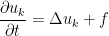
    \displaystyle \frac{\partial u_k}{\partial t}=\Delta u_k+f

    \displaystyle u_k|_{t=0}=u_0

    \displaystyle \frac{u_k}{\partial t}|_{\partial M_k}=0

    we know

    \displaystyle ||u(t)||_{C^0(M_k)}\leq ||u_0||_{C^0(M_k)}+t||f||_{C^0(M_k)}

    this is what Schauder estimate tell us.
    1.the uniform estimate with k:
    {||u_k||_{***}\leq C} independent of k.(now we do not know what the norm {||\cdot||_{***}} need to be)
    we have {C^0} estimate and the energy estimate as follows:
    from maximal principle,easy to get {C^0} norm estimate.

    the point is the equation {\frac{\partial }{\partial t}u_k= \Delta u_k +f} is strict parabolic so we have strong maximal principle and to construct suit bump function we can estimate {C^0} norm of {u_k}.

    from energy method we can estimate {\int_{M_k} ||\nabla u_k||^2}.

    the point is:
    {\frac{\partial}{\partial t}\int_{M_k} |\nabla u_k|^2=2\int_{M_k} \nabla u_k \cdot \frac{\partial}{\partial t}(\nabla u_k) }
    {=2\int_{M_k} \Delta u_k \cdot \frac{\partial}{\partial t} u_k }
    {=-2\int_{M_k}(\frac{\partial}{\partial t} u_k -f)\cdot \frac{\partial}{\partial t}u_k}
    {=-2[\int_{M_k}|\frac{\partial}{\partial t}u_k|^2-\int_{M_k} f\cdot \frac{\partial}{\partial t}u_k]}
    {=-2\int_{M_k}|\frac{\partial}{\partial t}u_k|^2-\int_{M_k}f \cdot (\Delta u_k +f)}
    {\leq 2\int_{M_k} \nabla u_k\cdot \nabla f}
    {\leq\int_{M_k} |\nabla f|^2 +\int_{M_k} |\nabla u_k|^2}.
    so we get:

    \displaystyle \frac{\partial}{\partial t}\int_{M_k}|u_k|^2\leq \int_{M_k}|\nabla f|^2+\int_{M_k} |\nabla u_k|^2

    so we can bounded {\int_{M_k}|u_k|^2}.
    for the general case:the equation becomes:
    \displaystyle \frac{\partial u}{\partial t}=a(x,t)\Delta u+b(x,t) \partial^i u+c(x,t)

    \displaystyle \frac{\partial u}{\partial v}|_{\partial M_k}=0

    \displaystyle u(0)=u_0

    but there is a hide Dragon,we need the condition {\frac{\partial u(0)}{\partial v}|_{M_k}=0}.
    otherwise we will get solution {u \notin W^{1,2}(M_k)\cap C^{2}(M_k)}.
    but in this case we still have the two necessary estimate(esay to see the above argument still make sense).
    in this case to prove the short time existence we need follow four claims is ture.
    \displaystyle ||u_{i+1,k}(t)||_C^0\longrightarrow ||u||_{i,k}{C^0}

    as {t \longrightarrow 0}
    \displaystyle \int_{M_k}|u_{i+1,k}|^2 \longrightarrow \int_{M_{k}}|u_{i,k}|^2

    as {t \longrightarrow 0}
    \displaystyle ||u_{i,k+1}(t)||_C^0\longrightarrow ||u||_{i,k}{C^0}

    as {t \longrightarrow 0}
    \displaystyle \int_{M_{k+1}}|u_{i,k+1}|^2 \longrightarrow \int_{M_{k}}|u_{i,k}|^2

    as {t \longrightarrow 0}
    5. Construct the suitable Banach space

    call the space construct follow the Mixed-Holder-Sobolev space for simply case,consider smooth manifold with only one conical singularity.
    first cover the whole manifold by a open set have positive distance t=with the conical singularity and a countable group of set {A_n=B(\frac{d}{2^n},p)-B(\frac{d}{2^{n+1}},p)},which is balls center at singularity {p} with radius {\frac{d}{2^n}}.(where {M=B(d,p)\cup U})
    i.e. {M-\{p\}=U \cup (\cup_{i=1}^{\infty}A_i)}

    Definition 2 ({||\cdot||_{\varepsilon^{k,\alpha}(S)}})
    \displaystyle ||f||_{\varepsilon^{k,\alpha}(S)}=sup_{k=1,2,...,\infty}||f(2^{-k},\theta)||_{C^{k,\alpha}(B_1-B_{\frac{1}{2}})}+||f||_{C^{k,\alpha}(U)}

    easy to see the definition is independent with the cover and the local interpolation coordinate chart.
    one thing is also trivial,is that we have the schauder estimate under the norm {||\cdot||_{\varepsilon^{k,\alpha}(S)}}.
    that is
    \displaystyle \delta u=f

    on {S-\{p\}}. {|u|<C_1} on {S}. then
    \displaystyle ||u||_{\varepsilon^{k+2,\alpha}}\leq C(||u||_{L^{\infty}}+||f||_{\varepsilon^{k,\alpha}})\leq C(C_1+||f||_{\varepsilon^{k,\alpha}})

    in fact we only need to add each inequality come from each open set of the cover by Schauder estimate to proof this.
    on the other hand we need a suitable Sobolev type norm.
    Definition 3 ({|\cdot|_w})
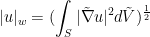
    \displaystyle |u|_w=(\int_S |\tilde \nabla u|^2d \tilde V)^{\frac{1}{2}}

    Definition 4 ({W^{k,\alpha}}) the set of all f in {\varepsilon^{k,\alpha}} with finite {|f|_w},
    \displaystyle ||f||_W^{k,\alpha}=||f||_{\varepsilon^{k,\alpha}}+|f|_w

    in Banach space.
    Assume norm {C^{k,\alpha}(B\times [o,T])} on {B\times [0,T]}

    Definition 5 ({||\cdot||_{\rho^{l,\alpha,{0,T}}}}]
    {f: S\times [0,T] \longrightarrow R }

    \displaystyle ||f||_{\rho^{l,\alpha,[0,T]}}=sup_{k=0,1,2,...,\infty}||f(2^{-k}\rho,\theta,4^{-k}t)||_{C^{l,\alpha}((B_1-B_{\frac{1}{2}})\times [0,4^{-k}T])}+||f||_{C^{l,\alpha}(U\times[0,T])}

    \end) from the definition,easy to see
    \displaystyle \frac{\partial u}{\partial t}=\Delta u+f

    om {M}
    \displaystyle u|_{t=0}=u_0

    {\Longrightarrow}
    \displaystyle ||u||_{\rho^{l+2,\alpha,[0,T]}}\leq C(||u_0||_{\varepsilon^{l,\alpha}}+||f||_{\rho^{l,\alpha,[0,T]}}+||u||_{C^0(S\times [0,t])})

    easy from the classical schauder estimate.

    Definition 6 ({|f|_v}) {f:S\times [0,T] \longrightarrow R}
    \displaystyle |f|^2_v=max_{t\in [0,T]}\int_S|\tilde \nabla f|^2d\tilde V +\int_0^T\int_M |\frac{\partial f}{\partial t}|^2 d\tilde Vd t

    Key point:

    Definition 7 ({\nu^{k,\alpha,{0,T}}}] {\nu^{k,\alpha,[0,T]}} is the set of {f} in {\rho^{l,\alpha,[0,T]}} with finite {|f|_v}
    \displaystyle ||\cdot||_{\nu^{k,\alpha,[0,T]}}=||\cdot||_{\rho^{l,\alpha,[0,T]}}+|\cdot|_v

    \end)
    6. What is a solution of equation

    trivial sense:
    satisfied equation point-wise on {S-\{p\}}.
    weak sense:
    1.trivial case
    2.{|u|_v<+\infty}


    补充说明

    以下是新整理的中文说明;上方旧博客原文保持不变。

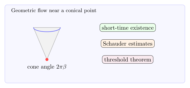
    几何流在光滑流形上已经有成熟理论,但一旦初始空间带有锥奇点,短时间存在和正则性都要重新组织。关键问题是:什么叫“光滑”,在哪个 Banach 空间中解方程,以及怎样在奇点附近建立 Schauder 型估计。

    锥奇点曲面上的几何流:短时间存在、Schauder 估计与阈值问题
    锥奇点附近的几何流需要在锥型 Holder 空间中建立短时间存在和 Schauder 估计。

    1. 锥奇点的局部模型

    在曲面上,锥角为 $2\pi\beta$ 的锥奇点可以局部写成

    $$g_\beta=dr^2+\beta^2r^2d\theta^2.$$

    若 $\beta=1$,这就是普通光滑点;若 $\beta\ne1$,度量在顶点处有角缺陷或角盈余。

    2. 几何流的困难

    Ricci flow、mean curvature flow、Calabi flow 等都可以写成抛物型方程。但在锥点附近,普通 Holder 空间不适合,因为坐标缩放和角变量的正则性发生改变。需要使用带权或锥型 Holder 空间。

    3. 短时间存在

    典型证明路线是构造映射

    $$T:A\to A$$

    其中 $A$ 是某个凸闭的函数空间球。若能证明 $T$ 连续、$T(A)$ 预紧并且 $T(A)\subset A$,就可以用 Schauder fixed point theorem 得到短时间解。

    4. Schauder 估计

    核心估计形如

    $$\|u\|_{C^{2+\alpha,1+\alpha/2}_\beta}\le C\bigl(\|Lu\|_{C^\alpha_\beta}+\|u\|_{C^0}\bigr).$$

    这里下标 $\beta$ 表示锥型空间。没有这类估计,固定点映射就无法闭合。

    5. 阈值型问题

    长期存在常常由某个阈值控制:只要解的 $L^\infty$ 或几何量保持有界,就可以继续延拓。锥奇点情形中,真正困难是证明这些控制不会在奇点附近丢失。

  • k-curvature 方程的 curvature measure 与可去奇点

    旧博客原文

    原题:k curvature方程的curvature测度和可去奇点的建立

    旧站归档中的这篇正文原本为空。


    补充说明

    以下是新整理的中文说明;上方旧博客原文保持不变。

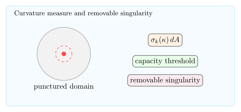
    对 $k$-curvature 方程,一个自然问题是:若解在孤立点或小集合上奇异,是否可以通过曲率测度判断这个奇点可去?这和调和函数的容量理论非常相似,只是曲率方程是完全非线性的。

    k-curvature 方程的 curvature measure 与可去奇点
    k-curvature 的可去奇点问题可以通过曲率测度是否在奇点集中携带质量来判断。

    1. 曲率测度

    若超曲面由图 $u$ 给出,主曲率为 $\kappa_1,\ldots,\kappa_n$,则 $k$-curvature 是

    $$\sigma_k(\kappa)=\sum_{i_1<\cdots

    对应的 curvature measure 可以理解为 $\sigma_k(\kappa)\,dA$ 的弱极限。即使 $u$ 不够光滑,这个测度仍可能有意义。

    2. 可去奇点的判据

    设 $u$ 在 $\Omega\setminus\{0\}$ 中满足方程。若奇点附近的曲率测度没有原子,或者其质量低于某个容量阈值,那么奇点往往可以去掉,$u$ 延拓为整个 $\Omega$ 上的弱解。

    3. 容量思想

    容量衡量一个集合对方程的影响。对 Laplace 方程,点在高维中可能容量为零;对 $k$-Hessian 或 $k$-curvature 方程,临界维数和 $k$ 有关。这决定了哪些奇异集合是“看不见”的。

    4. 建立理论的路线

    证明通常需要三步:先定义弱曲率测度;再证明光滑逼近下测度收敛;最后用比较原理和容量估计排除奇点处的额外质量。这样可去奇点问题就变成测度是否携带集中曲率。

  • Schrodinger 方程的衰减性估计:dispersive estimate 与 Strichartz

    旧博客原文

    原题:关于shordinger方程的衰减性估计

    旧站归档中的这篇正文原本为空。


    补充说明

    以下是新整理的中文说明;上方旧博客原文保持不变。

    自由 Schrodinger 方程

    $$i\partial_tu+\Delta u=0,\qquad u(0)=u_0$$

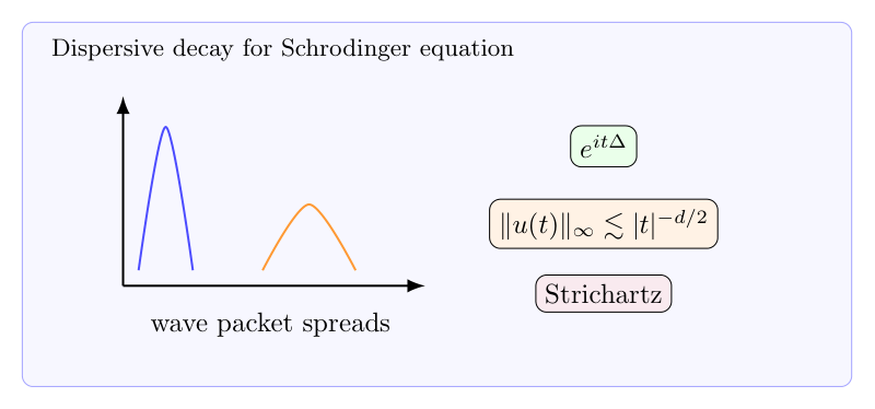
    的解为 $u(t)=e^{it\Delta}u_0$。衰减估计描述的是:初始波包随着时间扩散,点态振幅下降。

    Schrodinger 方程的衰减性估计:dispersive estimate 与 Strichartz
    Schrodinger 衰减估计来自自由传播核的二次振荡,进一步导出 Strichartz estimates。

    1. 核函数公式

    在 $\mathbb R^d$ 上,传播算子有显式核

    $$e^{it\Delta}u_0(x)=\frac1{(4\pi it)^{d/2}}\int_{\mathbb R^d}e^{i|x-y|^2/(4t)}u_0(y)\,dy.$$

    直接取绝对值得到 dispersive estimate:

    $$\|e^{it\Delta}u_0\|_{L^\infty}\le C|t|^{-d/2}\|u_0\|_{L^1}.$$

    2. 衰减来自振荡

    核的大小给出 $|t|^{-d/2}$,本质上是相位 $|x-y|^2/(4t)$ 的非退化二次振荡。高维中波包扩散到更大的空间体积,所以衰减更快。

    3. Strichartz 估计

    把 dispersive estimate 与 $L^2$ 守恒结合,通过 $TT^*$ 方法可以得到 Strichartz estimates:

    $$\|u\|_{L_t^qL_x^r}\le C\|u_0\|_{L^2},$$

    其中 $(q,r)$ 满足 Schrodinger admissible 条件。

    4. 非线性方程中的作用

    对非线性 Schrodinger 方程,衰减估计控制 Duhamel 项,使局部适定性、散射、小数据全局解等问题可以在函数空间中闭合。