We focus on , it does not mean is the only compact 1 dimensional system , but it is a typical example.
.
If is a homomorphism then stay the order of (by continuous and the zero point theorem). That is just mean:
(may be do a reflexion ).
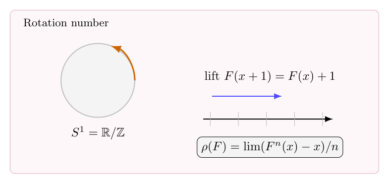
In the homomorphism case. We try to define the rotation number to describe the expending rate of the dynamic system.
i.e. . Lifting to,
.
How to realize the lifting?
Step1: Periodic extend to . (Regard as ).
Step2: Consider the “flow” of . we get .
The rotation number is defined as:
.
Following we will shall it is independent of the choice of and in fact.
It is not difficult to proved the following property:
Property:
1.If is conjugate (in fact semi-conjugate is enough ). Then 1.If is conjugate (in fact semi-conjugate is enough ). Thenrotation number of equal to rotation number of .
2.If is conjugate to . Then rotation number of equal to
rotation number of .
)
Example: , . It is not difficult to prove the rotation number of is .
Propersion:
1)For we have that .
2).If has a periodic point, i.e. . Then $latex\rho (T)$ is rational.
3) has no periodic point then is irrational.
4) The limit actually exists and we have: .
pf of 1):
.
Used the property .
pf of 2):
It is not difficult to prove is independent with the choice of . So choose to be the periodic point.
Remark: but the inverse of 2) is not true. For example:
.
This dynamic system has both periodic points() and non-periodic pint (maybe orbits generated by .
pf of 3):
If not. Assume is rational number . Take any point , then:
.
.
.
Now assume .
Then . $\forall x\in \mathbb S_1$ (if , take reflection ).
And there do not exists such that . If not, we could prove rotation number is large than lead a contradiction.
So is a bounded monotonically increasing sequences in , it limits point must satisfied .
pf of 4):
Using the point wise approximation inequality induced from the monotonically and stay ordering property of by .
Corollary:
Assume is irrational.
1. Let , and . If , then .
2. The bijection between the set and precise the natural ordering on .
This corollary is not difficult to prove use the established property.
Denjoy’s theorem
Proposition:
If is a minimal orientation presenving homomorphism with irrational rotation number then is topologically conjugate to the standard rotation .
leave as a ex.
For , . We define the variation of by:
We say that the logarithm of has bounded variation if this value is finite.
Denjoy’s theorem:
If is a orientation preserving homomorphism of the circle with derivative of standard variation and irrational rotation number then is topologically conjugate to the standard rotation :
.
Due to the upper proposition we only need show is minimal. Proof pf minimal is splitting to following two sub lemmas.
Sublemma1:
If has irrational rotation number and there are a constant and a sequences of integers such that the map: Satisfy : Then is minimal.
Sublemma2:
Fix and write , for There exists an increasing sequences of natural number such that the intervals are all disjoint.
Paradox and problem
Graph:
because of existence of fix point.
for .
Is always true for ?
If it is right, then there is a contradiction with argument , but for what type of dynamic system ?
satisfied . for all ?
Problem:
If is not homomorphism but induced , is striating increasing, Is the limit of always exists? it could not be increase with .
补充说明
以下是新整理的中文说明;上方旧博客原文保持不变。
rotation number 是一维动力系统中最基本的不变量之一。它衡量圆周同胚平均每次迭代旋转多少。
Where is a given periodic matrix with period , i.e. .
Then the solution $\phi(t)$ satisfied identity:
.
This could be explained as .
Now we consider to solve the equation: . At least formally it could be solved:
.
(Unfortunately is a multi-value function so , where is the identity matrix and is a solution of .) This argument is false.
In fact matrix is not like numbers, the function is much more complicated. we have,
So to solve , it is equivalent to :
But this type of identity only meaningful when , so is it true that for the equation is solved by , and for it do not have solution?
The naive inspirit is wrong, the situation is similar to the case while could extend to and the identity
always holds for . The key observation is always holds when , this will lead to a reasonable value of
even when and this process could be continue to the whole matrix space and the identity enjoy the accosted principle so is well-defined for all .
Now it is time to consider the rotation number, which is defined by for is a continuous increasing function.
And I do not know how to associated a dynamic system for the matrix given here, but in any case it seems iff it is given by a hemoermorphifm then the rotation number is zero due to the following reason:
Consider as the quotient . Your homeomorphism lifts to a homeomorphism
such that .
Form the map , where is the composition times of with itself. By construction and , so that factors as a homeomorphism of the circle conjugating to the rotation.
By the way this approach wors in too.
Maslov index of a holomorphic disk
A natural way to understand the rotation number here is according the way of maslov index, we have the following formula:
Proof sketch:
1..
2. The dynamic system is defined by : , .
3. this dynamic system is conjugate to the dynamic system , Not difficult to proof it is a homomorphism on and it is zero entropy by Pesin’s formula
If could lifting to $\hat T:R \to R$ the rotation number is defined as :
This problem is not a good problem due to the philosophy, i.e. use rotation number to describe the information of a hamiltonian flow is not satisfied, in fact it is difficult to establish a suitable definition of “rotation number”! But this is the first crucial thing to establish a theorem!
Hamiltonian flow
In mathematics and physics, a Hamiltonian vector field on a symplectic manifold is a vector field, defined for any energy function or Hamiltonian. A Hamiltonian vector field is a geometric manifestation of Hamilton’s equations in classical mechanics. The integral curves of a Hamiltonian vector field represent solutions to the equations of motion in the Hamiltonian form. The diffeomorphisms of a symplectic manifold arising from the flow of a Hamiltonian vector field are known as canonical transformations in physics and (Hamiltonian) symplectomorphisms in mathematics.[1]
Hamiltonian vector fields can be defined more generally on an arbitrary Poisson manifold. The Lie bracket of two Hamiltonian vector fields corresponding to functions f and g on the manifold is itself a Hamiltonian vector field, with the Hamiltonian given by the Poisson bracket of f and g.
补充说明
以下是新整理的中文说明;上方旧博客原文保持不变。
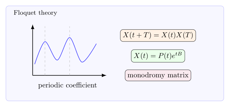
Floquet theory 研究周期系数线性微分方程
$$\dot x=A(t)x,\qquad A(t+T)=A(t).$$
它告诉我们,周期系统的长期行为由一个周期部分和一个指数部分共同决定。
Floquet theory 把周期系数线性系统分解成周期部分和指数部分,monodromy matrix 控制稳定性。
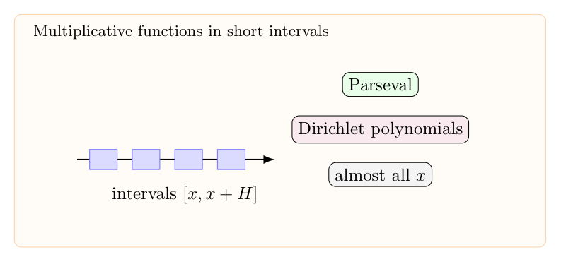
The most important beakgrouth of analytic number theory is the new understanding of multiplication function on share interval, this result is established by Kaisa Matomäki & Maksym Radziwill. Two very young and intelligent superstars.
The main theorem in them article is :
Theorem(Matomaki,Radziwill)
As soon as  when , one has:


for almost all  .
In my understanding of the result, the main strategy is:
Parseval indetity, monotonically inequality, this is something about the norms of the quality we wish to charge. It is just trying to understanding
as a fuzzy thing by a more chargeable quality:
In fact we do a cutoff, the quality we really consider is just:
established the monotonically inequality:
In my understanding, This is a perspective of the quality, due to the quality is a multiplicative function integral on a domain () with additive structure, it could be looked as a lots of wave with the periodic given by primes, so we could do a orthogonal decomposition in the fractional space, try to prove the cutoff is a error term and we get such a monotonically inequality.
But at once we get the monotonically inequality, we could look it as a compactification process and this process still carry most of the information so lead to the inequality.
It seems something similar occur in the attack of the moments estimate of zeta function by the second author. And it is also could be looked as something similar to the spectral decomposition with some basis come from multiplication unclear, i.e. primes.
Step 2: Involved by multiplication property, spectral decomposition
I called it is “spectral decomposition”, but this is not very exact. Anyway, the thing I want to say is that for multiplication function , we have Euler-product formula:
Euler-product formula:
But anyway, we do not use the whole power of multiplication just use it on primes, i.e. leads to following result:
This is a identity about the function , the point is it is not just use the multiplication at a point,i.e. , but take average at a area which is natural generated and compatible with multiplication, this identity carry a lot of information of the multiplicative property. Which is crucial to get a good estimate for the quality we consider about.
Step 3:from linear to multilinear , Cauchy schwarz
Now, we do not use one sets , but use several sets which is carefully chosen. And we do not consider [X,2X] with linear structure anymore , instead reconsider the decomposition:
On every it equipped with a bilinear structure. And is a very small set, $|U|=o(X)$ which is in fact have much better estimate.
This problem may be a embarrassed one, but I even could not prove it for the 1 dimensional case.
Here is the problem:
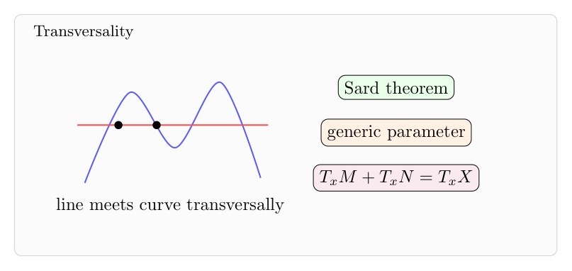
>**Question 1** is a compact -dimensional smooth manifold in , take a point $p\notin M$. prove there is always a line pass and , and intersect transversally with .
You can naturally generated it to:
>**Qusetion 2** is a compact $n$-dimensional smooth manifold in , take a point . Prove $\forall 1\leq k\leq m$, there is always a hyperplane pass $p$ and , and intersect transversally with .
Thanking for Piotr pointed out, assuming “transverse” means “the tangent spaces intersect only at 0”.
We focus on question 1 for simplified.
Even in 1 dimension it is not easy at least for me, **warning**: a line pass may be intersect $M$ at several points combine a set , could be finite, countable or even it is not countable (consider is induced by a smooth function for which the zeros set is Cantor set.)… And if there is one point , $l$ is tangent with the tangent line of at , then is not intersect transversally with .
**My attempt**:
I could use a dimensional argument and Sard’s theorem to establish a similar result but instead of a fix point , we proof for generic point in which is not in we can choose such a line.
So it seems reasonable to develop the dimensional technique to attach the question 1, in 1 dimensional, it will relate to investigate the ordinary differential equation:
Where , have a parameterization . If there is a counterexample for the question 1, then there is another solution which satisfied the ODE in the sense:
at least for every line there is a intersection point , satisfied ODE at .
This is just like the uniqueness of the solution of such a ODE is destroyed at some subspace of a line which have some special linear structure, I do not know if this point of view with be helpful.
I will appreciate for any useful answers and comments.
Proof 1(provided by fedja)
Area trick.(weakness:it seems we could not proof the transtivasally intersection point have positive measure by this way).
Proof 2(provided by Piotr)
#For the codimension 1 case.#
###Using Thom transversality theorem.###
Consider the maps parametrized by and given by . The map , is clearly transverse to , thus Thom’s transversality says that is transverse to for almost all . Now it suffices to prove that for an open set in , the line given by intersects . Proven below.
###Using Sard’s theorem directly.###
Thom’s transversality is usually proven using Sard’s theorem. Here is the idea.
Consider the projection onto a sphere centered at . A line through intersects transversally if the two points are regular values of (indeed, the critical points of are exactly the points at which the normal is perpendicular to the radial direction (with respect to $p$)). By Sard’s theorem, the set of regular values is dense in .
We need to choose any point on the sphere for which both and are regular values, and the line through and actually intersects . It suffices to prove that the set of points for which this line intersects contains an open set. We could now use the Jordan-Brouwer Separation Theorem and we would be done, but we can do it more directly (and in a way that seems to generalize).
###The set of points for which intersects has nonempty interior.###
For each point the projection onto the sphere centered at , of radius small enough so that the sphere does not intersect , has some (topological) degree . It is easy to check that if one takes any point and considers the points for small , the degrees of the corresponding maps differ by . It follows that we can find a point for which , which guarantees that for every point in a small open ball around (all these points have same degree ), the line joining and intersects . Projection of on is an open set which we sought.
#For the general case (partial solution).
I think a similar reasoning should work, however, notice that for we cannot make intersect transversally with because of dimensional reasons: the dimensions of and don’t add up to at least . Recall that transversality implies Thus, either (1) you want to consider , or (2) define “transversal intersection” for such manifolds saying that the tangent spaces have to intersect at an empty set.
Also, for we can just take any plane which works for and just extend it to a -dimensional plane.
###Assuming .###
A similar reasoning should work for with going over all families of pairwise perpendicular unit vectors, and . Thom’s transversality says that for almost all choices of , the plane is transverse to .
### The nonempty interior issue. ###
The only thing left is to prove that the set of for which the intersection is nonempty has nonempty interior. Last time we proved that there is a zero-dimensional sphere containing , namely , which has nonzero linking number with , and by deforming if to spheres and taking lines through pairs , we got an open set of parameters for which the line intersects .
Here should be able to do a similar trick by finding a -dimensional sphere with nonzero linking number with . The ball that bounds that sphere has to intersect , thus the plane containing the sphere has to intersect . By perturbing the sphere we get spheres with the same linking numbers, and get all the planes that lie in a neighbourhood of ; in particular, we get an open set of parameters for which intersects .
Well, we don’t actually need a *round* sphere, but we do need a *smooth* sphere that lies in a -dimensional plane. There’s some trickery needed to do this, but I am sure something like this can be done.
Maybe somebody else can do it better?
### For ###
I don’t really know how to attack this case, assuming “transverse” means “the tangent spaces intersect only at “.
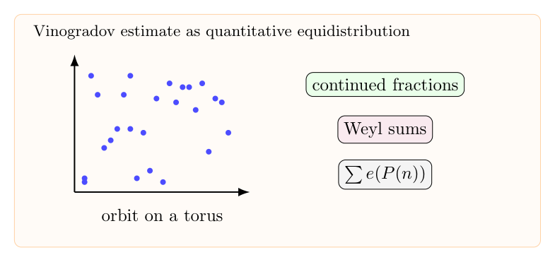
Assume , this could view as a effective uniformly distribute result of dynamic system: , where , is a nilpotent matrix, matrix is identity but with a irrational number in the elements.
First approach
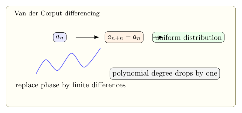
we could easily to get a “uniform distribute on fiber” result without very much tough estimate to attach the theorem. That is just a application by my “rigid trick” that is describe in my early note. But this approach is according to the understanding of the result as a uniformly distribute result on Torus , we could do this approach with the last , which will corresponding to , i.e. we could apply the “rigid trick” to prove sequences is uniformly distribute according to .
Graph
But this approach seems difficult to generate. The difficulty is come from both there is no similar uniformly distribute of the other perimeter use the rigid trick (At least as I know, I try to prove there could be one but I failed) and if in the best case we have the similar uniformly distribute result for other perimeter there is still some thing more need to be established. See this graph for a counterexample that the uniformly distribute for all fiberation could not derive a uniformly distribute for the original space.
Second approach
In this approach we need use the information of continue fractional to get some information (Which is of course critical to get some information about the estimate). But I do not know if it is necessary, maybe this could be a interesting question weather the information come from continue fractional must involve to get such a estimate in the future, but not today.
Any way, there is two different type of continue fractional:
1..
2..
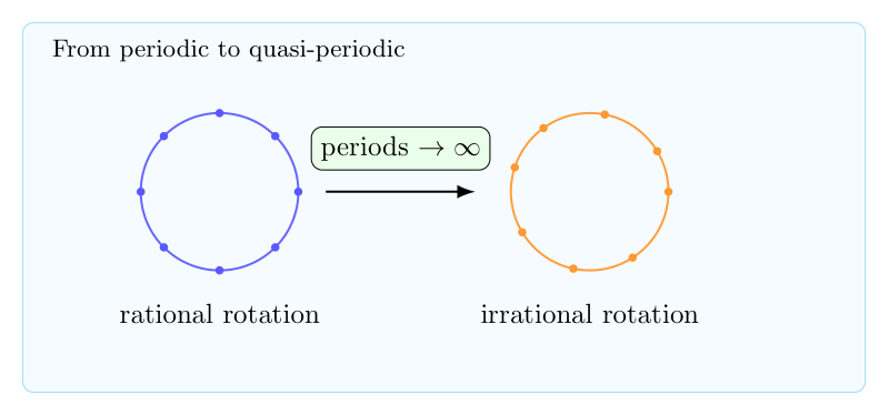
Anyway, these could be understand as a same thing more or less (if fact we can calculate some quantitive with which is roughly the same). That is just the orbits have quasi-period property, that is to say, under certain norms, it could be understand as the limits of periodic sequences. So it is natural to approximation by periodic sequences and will lead to a very good point-wise coverage result:
Where is just the periodic approximation sequence which come from the best approximation (critical point of ), which natural occur in continue fractional. And by this we already arrive a non qualitative form result of with .
But unfortunately this approximation is too good to be true for case. The reason of this result could be true is just because the natural estimate for the best approximation of ; i.e. Dirichlet approximation theorem.
But for higher degree case, although we could not expect this thing to be true, we still could image a weaker but enough result to be true:
in the Gromov Hausdorff metric sense, and the $T_k^n(x)$ is carefully chose, which have a finite torsion structure(which could be view as a multilinear structure which will play a central role in the estimate). Here is a graph for :
Roughly speaking, in general case, there is a cube structure in the orbits and is critical to observe that the progression of difference structure in it. The goal of this approach is to establish some result from the finite torsion structure(multilinear structure). That is to say, the boundary is high order thing in all direction but there is only one direction attend to infinity the other is just a finite torsion, and we wish to get more information from the extra structure.
This also have a physics explaining, for which see the graph:
原题:A discret to continuous approach to the Dirichlet principle.
Direchlet principle: is a compact set with $C^1$ boundary. then there exists unique solution $f$ satisfied $\Delta f=0$ in $\Omega$, $f=g$ on .
Perron lifting and barrier function
We know the standard approach of the Dirichlet principle is perron lifting and construction of barrier function on the boundary.
The key point is if we define the variation energy , then it is easy to see for is in perron set, . So we can begin from a maximization sequence to construct a Cauchy sequence by perron lifting and by the involve of barrier function to make the solution compatible with the boundary condition then arrive a proof.
But when I was a freshman in undergraduate school and I do not know the method of perron lifting I try something I name it from discret to continuous approach to try to solved the problem. It is always a puzzle in my mind iff we can solve the Dirichlet principle in this way, roughly speaking, it is divid into two part:
1. Investigate the discretization of harmonic function in smaller and smaller scale. The discretization I consider is just i.e. the -latties in $\Omega$,and discretization Laplace operator . Some result is much easier to arrive with the discretization thing, you know ,such as the existence of solution is just come from simple linear algebra. and we can deduce harneck inequality, gradient estimate, even green function. So we get a solution of discretization and we do a extension to by take value of a small tube by the center of the tube, where the value have a definition by , and now we get .
2. The second step is to proof the solution with -discretization problem will coverage to the solution of original problem;i.e. we want to proof a estimate;i.e. , we have , . and by Albano-Ascoli theorem to construct . Then we need to proof $f$ is the harmonic function we find, to verify this information we use the mean-value property. So we need to prove satisfied mean-value property for every ball in .
Here is my first question,
> **Question 1:** How to prove the estimate and the MVP of -discretization will coverage to the MVP in case occor in second step?
My attempt to the estimate is by renomelazation which seems could work, but the annoying thing is to proof the mean-value property will coverage to the real one, I try to use some result of random walk, but it seem not works…
My second question is:
> **Question 2:** Are this approach a universal phenomenon? At least could we use this approach to establish the existence of solution for linear elliptic and parabolic equation?
The Third question is:
> **Question 3:** If we consider some inverse problem, that is to say, form a MVP instead of a PDE to derive a solution, could this always be possible? some example is, if we change the mean value property for harmonic function from the average of ball to cube or triangle or elliptic or something else, what happen? Is there always a solution satisfied the news MVP point-wise? If not, Is there some counterexample? on another hand, if yes, are them came from some PDE?
补充说明
以下是新整理的中文说明;上方旧博客原文保持不变。
Dirichlet 原理说:给定边界值,调和函数是 Dirichlet energy 的极小者。除了 Perron 方法和 barrier function,也可以从离散问题逼近连续问题。
In 1911 year, when Weyl is a young mathematician specticlizing in integrable system and PDE, He proved the important result about the asystomztion of eigenvalues of Dirichelet problem in is a compact domain;i.e.
Which in fact is a conjecture of *** in *** in published in 1910.
This is definitely a very amazing achievement of mathematician, The realist meaning we can actually charge with the spectrum asyspesion.
In fact, we know, the only thing we know is that the eigenfunction with different spectrum is orthogonal and we have are a cretition named maximum-minmum principle for the k eigenvalue. but how could we charge with the asymotum of them? It seems not to be chargeable, though we have a isometry, the spectrum expansion, ut it still not seems to be chargeable the main difficult come from the compacness this just mean a divide of the whole space, and we consider the X-ray tansigation from every point to the whole space, it need to be passion kernel, or we change it to be a pare matrix.
Yes, We can just look this phenomenon as there are two different world, one is the real world in the Ecliud space, there other is the a wave function world, in the second world it is composted by the unique of the solution for for some eigenvalue and all units in this world is the translation and rescaling of u. Then thing become interesting, now how to understand the other guy, i.e. the other eigenvalue and eigenfunctions? They must be the u after some translation combine with rescaling and trslation and rotation!!! so there is a dynamic system action on it! and if we only let it to be affine map,i.e. combine only taslation and rotation, then we just get the all eigenfunctions with the same eigenvalue.
Now let us see what is it, it is just need to be compatible with the boundary condition, so it need to be moduli space that the boundary map is a measure that is arrive able by only affine translation of the function (we look it as a obsevalbel) So it is a restriction from a high dimensional space to the boundary of it. and very fortunately it could assume a
补充说明
以下是新整理的中文说明;上方旧博客原文保持不变。
Weyl law 描述 Laplace 算子特征值的渐近分布。它说明高频谱的主要项只看区域体积和相空间体积,而不看边界的细节。
Weyl law 把 Laplace 特征值计数的主项解释为 phase space volume。
原题:Sarnak conjecture, understand with standard model
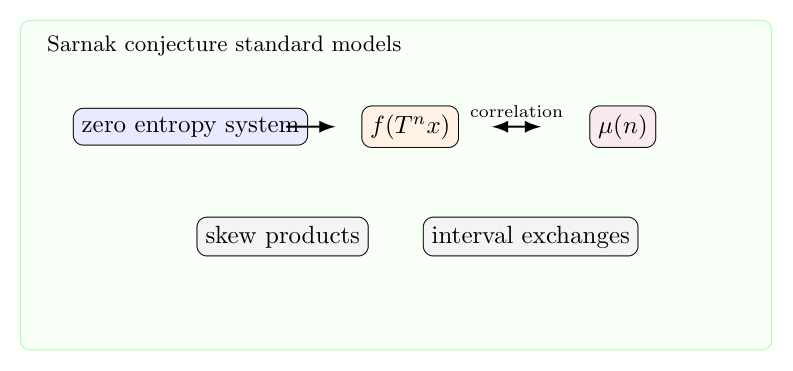
Sarnak conjecture is a conjecture lie in the overlap of dynamic system and number theory. It is mainly focus on understanding the behavior of entropy zero dynamic system by look at the correlation of an observable and the Mobius function .
We state it in a rigorous way:
let be a entropy zero topological dynamic system. Let Mobius function be defined as , where $latex$ is the number of different primes occur in the decomposition of .
Then for any continuous function and , observable is orthogonal to the Mobius function; i.e. ,
by Bourgain-Ziegelar-Sarnak theorem we know the difficulties is focus on deal with the exponent
for all is suffice large primes pair.
and a much simper case is the affine map: on and the general case where A is a upper-triangle matrix with diagonal 1; i.e. , B is nilpotent. So the sarnak conjecture in this case is reduce to the Davenport estimate on exponent by B-Z-S theorem:
, .
Interval exchange map
For the interval exchange map, we can explain it by a composition of rotation of some part of step by step and with a renormalization process to glue the neighbor rotations.
Now let us explain a little with this interesting dynamic system. We focus in the simplest nontrivial case, which is the 3-interval exchange map. In this case, just consider the permutation of intervals , and it is easy to see there is only one case is nontrivial that is permutation: . We explain a little more with other trivial case:
When , the interval exchange map is just a rotation and for which the sarnak conjecture is just come from:
, .
Which is trivial because .
For the case $I_1\to I_2, I_2\to I_1, I_3\to i_3$ the map is a rotation on but it is a identity map on and the orbits of point only lying one of $I_1\cap I_2, I_3$, lying in which one depend on the original point we take is lying in which one.
Now we focus on the most difficult situation. It is annoying but it is the obstacle we must get over to go far. Fortunately it could be explained as in the following picture.
3-Interval exchange map as two rotation map glue with a renormalization map.
Now we explain what happen in the picture, it is mainly say one identity, which explain how to look 3-interval exchange map as a composition of rotation map with a renormalization map to glue them. Rotation is a kind of map we have good understanding but we do not understand very well with the renormalization map which is glue the two endpoints of which are not the common endpoint of them. Then you get two circle glue like a “8” , and is just rotate one of it and make the other one to be invariance.
Now we roughly could think about what is the thing we need to charge with, it is just:
.
Now we do some calculate with this geometric explain of interval exchange map.
Let , then . And , . the rotation , .
Standard model
Is there a standard model of entropy zero dynamic system?
This problem seems to be too ambitious. But it occur naturally when I an trying to have a global understand of the Sarnak conjecture.


![[0,2\pi]](https://s0.wp.com/latex.php?latex=%5B0%2C2%5Cpi%5D&bg=ffffff&fg=5e5e5e&s=0&c=20201002)


is conjugate (in fact semi-conjugate is enough ). Then 1.If


we have that
.
. Then $latex\rho (T)$ is rational.
has no periodic point then
is irrational.
.






, and
. If
, then
.
between the set
and
precise the natural ordering on
.
is a minimal orientation presenving homomorphism with irrational rotation number
then
.






orientation preserving homomorphism of the circle with derivative of standard variation and irrational rotation number
then
.
and a sequences of integers
such that the map:
Then
and write
, for
There exists an increasing sequences
are all disjoint.


is not homomorphism but
induced
,
is striating increasing, Is the limit of
always exists? it could not be increase with

 is a given periodic matrix with period
  .
. .
. .
. . At least formally it could be solved:
 .
. is a multi-value function so
  , where
  is the identity matrix and
  is a solution of
 , it is equivalent to :
 , so is it true that for
  it do not have solution?
 case while
  could extend to
  and the identity
 . The key observation is
 ![log[(1+Y)(1+Y)]=log(1+X)+log(1+Y)](https://s0.wp.com/latex.php?latex=log%5B%281%2BY%29%281%2BY%29%5D%3Dlog%281%2BX%29%2Blog%281%2BY%29&bg=ffffff&fg=5e5e5e&s=0&c=20201002) always holds when
always holds when  , this will lead to a reasonable value of
![log[(1+X)(1+Y)]=log(1+X+Y+XY)](https://s0.wp.com/latex.php?latex=log%5B%281%2BX%29%281%2BY%29%5D%3Dlog%281%2BX%2BY%2BXY%29&bg=ffffff&fg=5e5e5e&s=0&c=20201002)
 and this process could be continue to the whole matrix space and the identity enjoy the accosted principle so
  is well-defined for all
  .
. for
for  is a continuous increasing function.
 as the quotient
  . Your homeomorphism
  lifts to a homeomorphism
 such that
  .
. , where
  is the composition
  times of
  with itself. By construction
  and
and  , so that
  factors as a homeomorphism of the circle conjugating
  too.
too.

 .
. ,
,  .
. is conjugate to the dynamic system
  , Not difficult to proof it is a homomorphism on
 in
in  ,
,  is uniformly distributed, then




 :
Given
:
Given  ,
,  coverages
to a uniformly distribution in
coverages
to a uniformly distribution in  as
as  .
.

 is true for
  .
.
 when
when  , one has:
 for almost all
  .
. norms of the quality we wish to charge. It is just trying to understanding


 ) with additive structure, it could be looked as a lots of wave with the periodic given by primes, so we could do a orthogonal decomposition in the fractional space, try to prove the cutoff is a error term and we get such a monotonically inequality.
 , we have Euler-product formula:
 leads to following result:
 , but take average at a area which is natural generated and compatible with multiplication, this identity carry a lot of information of the multiplicative property. Which is crucial to get a good estimate for the quality we consider about.
 which is carefully chosen. And we do not consider [X,2X] with linear structure anymore , instead reconsider the decomposition:
![[X,2X]=\amalg_{i=1}^n (I_i\times J_i) \amalg U](https://s0.wp.com/latex.php?latex=%5BX%2C2X%5D%3D%5Camalg_%7Bi%3D1%7D%5En+%28I_i%5Ctimes+J_i%29+%5Camalg+U&bg=ffffff&fg=5e5e5e&s=0&c=20201002)
 it equipped with a bilinear structure. And
  is a very small set, $|U|=o(X)$ which is in fact have much better estimate.
 is a compact
  , take a point $p\notin M$. prove there is always a line
  pass
pass  and
and  , and
, and  , take a point
  . Prove $\forall 1\leq k\leq m$, there is always a hyperplane
  pass $p$ and
  , and
, and  intersect transversally with
  pass
pass  ,
,  , $l$ is tangent with the tangent line of
  , then
 ,
,  . If there is a counterexample for the question 1, then there is another solution which satisfied the ODE in the sense:
 ,
,  .
. parametrized by
  and given by
  . The map
  ,
,  is clearly transverse to
  is transverse to
  . Now it suffices to prove that for an open set in
  , the line given by
  onto a sphere centered at
  are regular values of
  (indeed, the critical points of
  at which the normal
  is perpendicular to the radial direction (with respect to $p$)). By Sard’s theorem, the set of regular values is dense in
  .
. are regular values, and the line
  for which
  the projection
  onto the sphere centered at
  , of radius
  small enough so that the sphere does not intersect
  . It is easy to check that if one takes any point
  for small
  , the degrees of the corresponding maps differ by
  . It follows that we can find a point
  , which guarantees that for every point
  in a small open ball
  is an open set which we sought.
 we cannot make
  . Recall that transversality implies Thus, either (1) you want to consider
  , or (2) define “transversal intersection” for such manifolds saying that the tangent spaces have to intersect at an empty set.
 we can just take any plane
  and just extend it to a
  -dimensional plane.
 .###
.### with
with  going over all families of pairwise perpendicular unit vectors, and
  . Thom’s transversality says that for almost all choices of
  , which has nonzero linking number with
  and taking lines through pairs
  , we got an open set of parameters for which the line intersects
  -dimensional sphere with nonzero linking number with
  containing the sphere has to intersect
  -dimensional plane. There’s some trickery needed to do this, but I am sure something like this can be done.
 ###
### “.
“.

 .
. , this could view as a effective uniformly distribute result of dynamic system:
 ![([0,1]^n,T)](https://s0.wp.com/latex.php?latex=%28%5B0%2C1%5D%5En%2CT%29&bg=ffffff&fg=5e5e5e&s=0&c=20201002) , where
, where  ,
,  is a nilpotent matrix, matrix
  is identity but with a irrational number
  elements.
 , we could do this approach with the last
  , which will corresponding to
  , i.e. we could apply the “rigid trick” to prove sequences
  is uniformly distribute according to
  .
. .
. .
. which is roughly the same). That is just the orbits
  have quasi-period property, that is to say, under certain norms, it could be understand as the limits of periodic sequences. So it is natural to approximation
 is just the periodic approximation sequence which come from the best approximation (critical point of
  ), which natural occur in continue fractional. And by this we already arrive a non qualitative form result of
  .
. case. The reason of this result could be true is just because the natural estimate for the best approximation of
 :
: and is critical to observe that the progression of difference structure in it. The goal of this approach is to establish some result from the finite torsion structure(multilinear structure). That is to say, the boundary is high order thing in all direction but there is only one direction attend to infinity the other is just a finite torsion, and we wish to get more information from the extra structure.
 case:
case:
 is a compact set with $C^1$ boundary. then there exists unique solution $f$ satisfied $\Delta f=0$ in $\Omega$, $f=g$ on
  .
. , then it is easy to see for
  is in perron set,
  . So we can begin from a maximization sequence to construct a Cauchy sequence by perron lifting and by the involve of barrier function to make the solution compatible with the boundary condition then arrive a proof.
 i.e. the
  -latties in $\Omega$,and discretization Laplace operator
  . Some result is much easier to arrive with the discretization thing, you know ,such as the existence of solution is just come from simple linear algebra. and we can deduce harneck inequality, gradient estimate, even green function. So we get a solution
  of
of  by take value of a small tube by the center of the tube, where the value have a definition by
  .
. estimate;i.e.
  ,
,  we have
  ,
,  . and by Albano-Ascoli theorem to construct
  case occor in second step?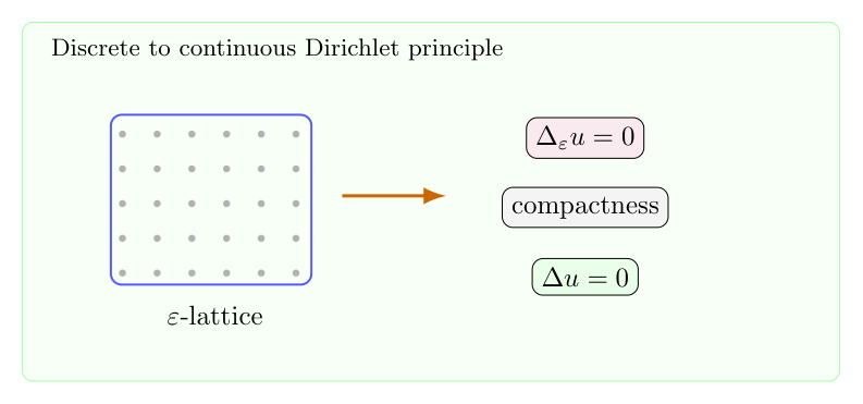
 is a compact domain;i.e.
 for
for  for some eigenvalue
  and all units in this world is the translation and rescaling of u. Then thing become interesting, now how to understand the other guy, i.e. the other eigenvalue and eigenfunctions? They must be the u after some translation combine with rescaling and trslation and rotation!!! so there is a dynamic system action on it! and if we only let it to be affine map,i.e. combine only taslation and rotation, then we just get the all eigenfunctions with the same eigenvalue.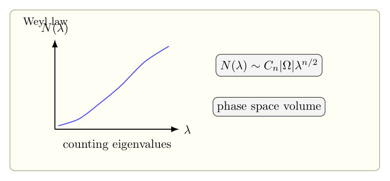
 be a entropy zero topological dynamic system. Let Mobius function be defined as
  , where $latex$ is the number of different primes occur in the decomposition of
  and
and  , observable
  is orthogonal to the Mobius function; i.e. ,
 is the skew product on
![[0,1]](https://s0.wp.com/latex.php?latex=%5B0%2C1%5D&bg=ffffff&fg=5e5e5e&s=0&c=20201002) .
. ,
, :
:
 , where
  .
.
 is suffice large primes pair.
 on
on  and the general case
  where A is a upper-triangle matrix with diagonal 1; i.e.
  , B is nilpotent. So the sarnak conjecture in this case is reduce to the Davenport estimate on exponent by B-Z-S theorem:
 ,
,  .
. , and it is easy to see there is only one case is nontrivial that is permutation:
  . We explain a little more with other trivial case:
 , the interval exchange map is just a rotation and for which the sarnak conjecture is just come from:
 ,
,  .
. .
. but it is a identity map on
  and the orbits of point only lying one of $I_1\cap I_2, I_3$, lying in which one depend on the original point
 which are not the common endpoint of them. Then you get two circle glue like a “8” , and
  is just rotate one of it and make the other one to be invariance.
 .
. , then
 ![A\cap B=\emptyset, A\cup B=[0,1]](https://s0.wp.com/latex.php?latex=A%5Ccap+B%3D%5Cemptyset%2C+A%5Ccup+B%3D%5B0%2C1%5D&bg=ffffff&fg=5e5e5e&s=0&c=20201002) . And
. And  ,
,  . the rotation
  ,
,  .
.