This is also true for . and the transform and permutation a classical result of markov claim that all solution of (*) could be generated from . I get a similar result for a similar algebraic equation 1 half years ago when consider a version of problem about 1-form given by Xu Bin.
Now we know the graph with root and with node generate by transform is connected.
The B-B-G-S conjecture is is the connected property still true for prime surfficed large?
补充说明
以下是新整理的中文说明;上方旧博客原文保持不变。
Markov triples 是方程
$$x^2+y^2+z^2=3xyz$$
的正整数解。经典 Markov 定理说,从根解 $(1,1,1)$ 出发,反复使用 Vieta involution
$$(x,y,z)\mapsto (x,y,3xy-z)$$
以及坐标置换,可以生成所有正整数解。
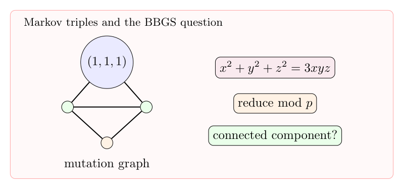
Markov triples 的 Vieta involution 生成解图;模 p 后的问题变成有限域曲面上的连通性问题。
1. 解图
把每个解看作图的一个顶点,若两个解由一次 Vieta involution 或置换相连,就连一条边。整数正解形成一棵以 $(1,1,1)$ 为根的巨大图。
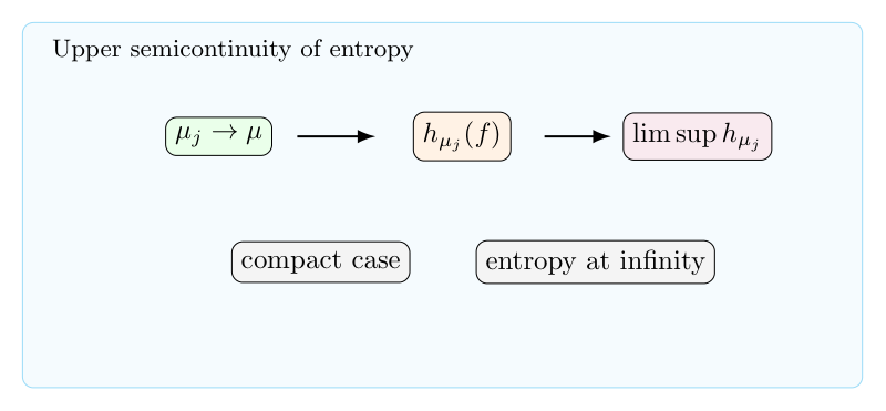
Now we focus on the upper semi-continuouty of the metric entropy map. The object we investigate is , where is a invariant measure.
The insight to make us interested to this kind of problem is a part of variational problem, something about the existence of certain object which combine a certain moduli space to make some quantity attain critical value(maximum or minimum). The most simple example maybe Isoperimetric inequality and Dirichlet principle of Laplace. Any way, to establish such a existence result a classical approach is to proof the upper semi-continuouty and bounded for associate energy of the problem. In our case the semi-continuouty will be some thin about the regularity of the entropy map:
We define the entropy at infinity:
Where varies in all sequences of measure coverage to in the sense for all , measurable then .
Compact case
we say some thing about the compact case, In this case we have finite partition with smaller and smaller cubes, this could be understand as a sequences of smaller and smaller scales. A example to explain the differences is , shift map on countable alphabet.
Because of this thing, there is a good sympolotic model, i.e. h-expension, and it generalization asymptotically h-expension equipped on a compact metric space $X$ have been proved to be that the corresponding entropy map is upper semi-continous.
In particular diffeomorphisms on compact manifold is asymptotically h-expensive.
Natural problem but I do not understand very well:
Why it is natural to assume the measure to be probability measure in the non-compact space?
Non-compact case
metric space
is a continuous map.
, then is still a metric.
Easy to see . This identity could be proved by the cretition of entropy by -seperate set and -cover set.
Kapok theorem:
compact, for every ergodic measure the following formula hold:
.
Where is the measure theoretic entropy of .
Riquelme proved the same formula hold for Lipchitz maps on topological manifold.
Let defined the moduli space of -invariant portability measure.
Let defined the moduli space of ergodic -invariant probability measure.
Simplified entropy formula:
satisfied simplified entropy formula if surfaced small and , .
Some basic thing, include the definition of metric entropy is introduced in my early blog.
Among the other thing, there is something we need to focus on:
1.Definition of metric entropy, and more general, topological entropy.
2.Spanning set and separating set describe of entropy.
3.amernov theorem:
.
Now we state the result of Margulis and Ruelle:
Let be a compact riemannian manifold, is a diffeomorphism and is a -invariant measure.
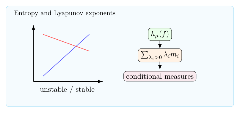
Entropy is always bounded above by the sum of positive exponents;i.e.,
Where is the multiplicity of and .
Pesin show the inequality is in fact an equality if and is equivalent to the Riemannian measure on . So this is also sometime known as Pesin’s formula.
F.Ledrappier and L.S.Young generate the result of Pesin.
One of their main result is:
is a diffemoephism, where is a compact riemanian manifold, f is compatible with the Lesbegue measure on , and
If and only if on the canonical defined quation manifold $M/W_{\mu}$, i.e. the manifold mod unstable manifold $W_{\mu}$, the induced conditional measure is absolute continuous.
Remark: according to my understanding, the equality just mean in some sense we have the inverse estimate:
This result maybe just mean near the fix point of ,i.e. the place charge the topology of the foliation, we have the inverse estimate. Such a inverse estimate will lead a control of the singularity of the push forward measure on the quation manifold. So have good regularity. But this idea is not complete to solve the problem.
Now we begin to get a geometric explain and which will lead a rigorous proof of the inequality:
At first we could observe that the long time average of could be diagonal. Assume after diagonal the eigenvalue is
.
This eigenvalue could divide into 3 parts: <0,=0,>0.
This will lead to a direct sum decomposition of the tangent bundle :
Where $E_u$ is the part corresponding to the eigenvalue>0, For this part we consider the more refinement decomposition:
, is the eigenvector space of . The dimension of $V_k$ is $dim V_k$.
On the other hand, we have a equality of metric entropy:
.
For the later one, is a measurable partition of , then could always be refine to a smaller partition , and we have:
.
Now we arrive the central place of the proof:
every partition could be refine by a partition with boundary of almost all cubes is parallel to the foliation. So we focus ourselves on the portion and all boundary of cubes in is parallel to the eigenvector.
Under this situation, we need only estimate the numbers of . Estimate it is not very difficult. we need only observe the following two thing:
1.
exists a.e. in . So this lead to the definition of foliation almost everywhere, and except a measurable zero set. In fact this set is the set of fix point of under .
2.
After a rescaling, every point which is not a fix point of could be understand as it is far away from fix points. Then the foliation could be understand as a product space locally. The flow with the direction which the eigenvalue is less than 1 cold not change . The direction with eigenvalue equal to 1 is just transition and just change the number of with polynomial growth. But the central thing is the direction with eigenvalue large than one and will make change with viscosity . and we product it and get :
Try beginning with Bendixon-Poincaré theorem, which is classical stuff and belongs to a lot of textbooks on vector fields.
Affine invariance
The number of limit cycle is invariant under affine map.
Classification of singular point
Bezout theorem
Example
1..The graph is just like:
2..The graph is just like:
3..The graph is just like:
4..The graph is just like:
5..The graph is just like:
6.. The graph of it is just like:
Now we try to explain the phenomenon we see. At first we can see there is no limit cycle in the picture. The bifurcation place is just the place and is just like 3 lines. And there are two singularity .
7.
8.:
9.:
exist 2 limits cycles.
10.
Tree structure
In general, the lower bound of is established. first by Otrokov,and later proved to be .
If right, this upper bound estimate is combine of two things:
1.every limit cycle do not intersect.
2.every unclear limit cycle contain a singularity.
Rough strategy attack Hilbert 16th problem
Step1:
The first step is to do some simplify, we know the number of limit cycles do not change under a affine map , where A is a nonsingular 2*2 matrix. So we could classify the topological graph of the dynamic system.
Step2:
Classification the singularity under affine map, and investigate the topological graph of the topological graph of the singularity by floer cohomology. There is only finite type and we could focus on them one by one.
Every color in the graph is an area $P,Q$ do not have same component in it. And the boundary of areas is just the same component of if it exists.
Step3:
Bezout theorem tell us if two polynomials do not have same connected component then the intersection . And we can divide the space into finite parts, restrict to every part do not have the same component. And we have a upper bound control on the number of part when . A easy arrive bound could be .
Step4:
Now we focus ourself on 1 part where do not have same component on it. Now we begin to proof there will be a relationship between the limit cycle, very like a tree structure, it will combine with the following two thing:
Every limit cycle contains at least one singularity or one smaller limit cycle inside it.
2. Every pair of limit cycle , are limit cycle and is inside of , then there is at least one singularity or another limit cycle contain in .
This kind of topological result will lead to a upper bound of number of limit cycle and end the proof of Hilbert 16th problem.
Planar polynomial vector field for a harmonic pair of polynomials
In this case you can consider the heat equation . If the number of the limit cycle change, it must be the time to pass a singularity. and take , the dynamic system coverage to a very simlpe one and in particular it do not have limit cycle. So we need only look at the moments passing singularity.
Has the system of ODEs:
been studied for the special case of the polynomials and being a harmonic pair, i.e. the real and imaginary part of a holomorphic polynomial , ?
I am looking to learn a bit about (complex) ODEs and their interplay with algebraic geometry by some examples, but I couldn’t find anything on this special case in Ilyashenko’s survey on Hilbert 16 (I guess this case is too special and/or not very interesting as far as Hilbert 16 is concerned).
Nontheless, it seems very natural. If we set , this amounts to the equation $latex \int_{\gamma_t}\frac{dz}{F(z)}=t$
where is the curve “truncated” at and the RHS is in particular **real**. This can be taken further, for example by assuming is closed and using the residue theorem to obtain constraints on (the coefficients of) .
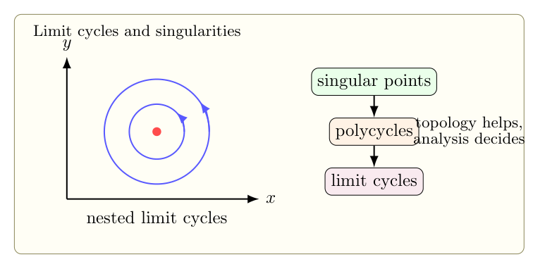
First, this case is totally uninteresting regarding Hilbert XVI. Indeed, there are no limit cycles in such systems. The -limit of a trajectory is either a point or a non-isolated cycle (center case).
A singularity at (*i.e.* a root of $F$) can only be of three types, according to the value of :
1. Source/focus: .
2. Center: .
3. Flower with petals: with multiplicity .
In addition there is a pole at infinity (if ) with exactly separatrices, reaching the singularity in finite time. The bassins of attraction / center regions attached to the above singularities are delimited by the separatrices.
[![enter image description here][2]][2]
S. Smale began to get interested in the question in the early 80’s while laying the foundations for BSS computational model (*The fundamental theorem of algebra and complexity theory*, 1981). He proposed a numerical root solver for polynomials by following the flow of . This started some works on the topic, for instance by Schub, Tischler, William (*The Newtonian graph of a complex polynomial*, 1988) or Benzinger (*Plane autonomous systems with rational vector fields*, 1991)…
In the case of these vector fields, the topological class is entirely encoded by their Newtonian graph (or the «dual» spinal graph) given by the incidence graph of the -limits of trajectories (in red on the picture). The main result for polynomials is that it is a tree. See *e.g.* Sverdlove (*Inverse problems for dynamical systems*,1981) and Schecter, Singer (*A class of vectorfields on $\mathbb S^2$ that are topologically equivalent to polynomial vectorfields*,1985) and Jongen, Jonker, Twilt (*On the classification of plane graphs representing structurally stable rational Newton flows*,1991).
The conformal classification has been initiated by Douady, Estrada and Sentenac (unpublished monograph, 2005) for the generic case (only focus/source singularities) and completed by Branner and Dias (*Classification of complex polynomial vector fields in one complex variable*, 2010). In addition to the combinatorial (topological) invariant, a complex «time-shift» (related to the integrals ) is associated to the separatrices, providing a complete conformal invariant.
In that latter context, the function is called a Fatou coordinates. It is a rectifying chart for the vector field, and has many interesting dynamical properties.
Notice also the deep and beautiful relationship between spinal graph and *Dessins d’enfants*, as established by Pilgrim (*Polynomial vector fields, dessins d’enfants, and circle packings*,2006), related to [this question](https://mathoverflow.net/questions/118527).
Classification of the singularity in even degree case.
Adjoint harmonic case have been studied. Look into the recent paper
Langley, J. K. Trajectories escaping to infinity in finite time. Proc. Amer. Math. Soc. 145 (2017), no. 5, 2107–2117, and the reference list in this paper.
They were also studied by physicists:
Bender, Carl M.; Hook, Daniel W.
Complex classical motion in potentials with poles and turning points.
Stud. Appl. Math. 133 (2014), no. 3, 318–336.
EDIT. I forgot to mention this:
B. Branner, K. Dias, Classification of complex polynomial vector fields in
one complex variable, Journal
Journal of Difference Equations and Applications
Volume 16, 2010 – Issue 5-6:
I see a similar formula I wish to be true and merely have a proof in mind occur as a MO’s problem:
In my research, I encounter the following formula which I believe is correct (checked for ). Is it classical ?
I am given a real symmetric matrix
where is a probability and .
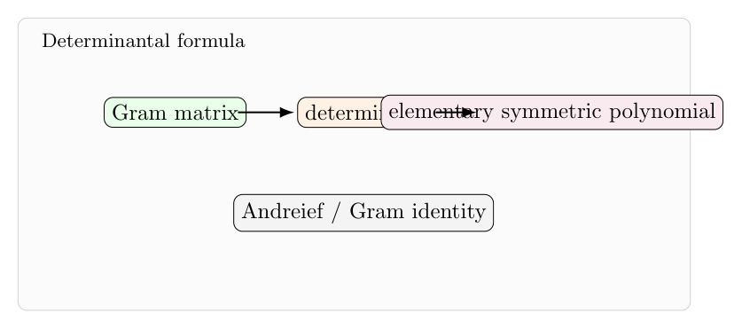
Let be the elementary symmetric polynomial in the eigenvalues of . For instance, is the trace and the determinant. The following formula gives in terms of the Gram matrix whose entries are the scalar products .
Remark that is positive semi-definite. The integrand is non-negative, as well as . The integrand vanishes identically iff takes values in a subspace of dimension , which is the condition under which vanishes. It follows that, if the formula above failed, it would be because of an inequality between strictly positive numbers.
The case is a consequence of the identity
which I have seen under the names “Andreief identity” and also “Gram identity”. The proof is elementary using the Leibniz formula for the determinant.
the statement go isometry inequality is very simple:
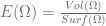
, iff is a ball, arrive a minimum .
This is a classical problem in variation theory. The difficult is divide into two parts. The first is to create a “flow” which descrement the energy and the “flow” is compatible with the feature of a ball, i.e. every set under the flow will tend to like a “ball”. The second one is to proof there exist a unit in the space make the Energy arrive a minimum.
Combine this two property we can consult that ball is the set and definitely the only set make the arrive the minimum.
first difficulties
The energy $E(\Omega)$ is scaling invariance. The first difficult could divide into two part:
Restrict to convex set
the first is to deform a set into a convex set and proof this process would not lower . This could been a little subtle. and the way I image could make sense is just like the following transform:
but this process is harder in higher dimension, for example:
Convex set to a ball
Steiner symmetric process.
Affine transform
Minkowski–Steiner formula
In mathematics, the Minkowski–Steiner formula is a formula relating the surface area and volume of compact subsets of Euclidean space. More precisely, it defines the surface area as the “derivative” of enclosed volume in an appropriate sense.
The Minkowski–Steiner formula is used, together with the Brunn–Minkowski theorem, to prove the isoperimetric inequality. It is named after Hermann Minkowski and Jakob Steiner.
Statement of the Minkowski-Steiner formula
Let , and let be a compact set. Let denote the [[Lebesgue measure]] (volume) of . Define the quantity by the ”’Minkowski–Steiner formula”’:
where:
denotes the [[closed ball]] of [[radius]] , and:
is the [[Minkowski sum]] of $latexA$ and , so that:
.
Surface measure
For “sufficiently regular” sets , the quantity does indeed correspond with the -dimensional measure of the [[boundary (topology)|boundary]] of . See Federer (1969) for a full treatment of this problem.
Convex sets
When the set is a [[convex set]], the [[limit inferior|lim-inf]] above is a true [[Limit of a sequence|limit]], and one can show that
:,
where the are some [[continuous function]]s of (see [[quermassintegral]]s) and $\omega_{n}$ denotes the measure (volume) of the [[unit ball]] in :
:,
where denotes the [[Gamma function]].
==Example: volume and surface area of a ball==
Taking gives the following well-known formula for the surface area of the [[sphere]] of radius , :
To establish a continue property of the Energy functional .
the continuous property is consider with all open set with Gromov-Hausdorff metric .
We need to proof the continuous of with the Gromov-hausdorff metric on the space consist with convex open sets.
To remark,we need to observe that polygon approximation is just corresponding to the points approximation in Gromov-hausdorff distance. and definitely carefully refinement of this kind of approximation could lead to the result of continuous of the energy on convex set.
A second remark, we definitely need a definition of the it could be achieve with open convex set by a outer and inter approximation by polygon and the error term estimate.
here is the problem, how to understand k-hessian equation and k-curvature equation.
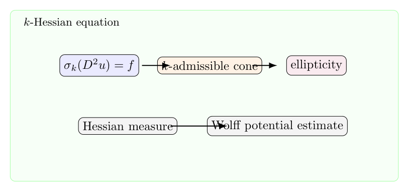
k-hessian equation
k-hessian equation is:
(*)
where u is admissible, i.e. , . this is just the condition to make (*) be a elliptic equation.
The most important result is the following three:
1.sovable (*) with direchlet boundary condition.
This is mainly the contribution of Caffaralli in 90’s. According flexible function and maximum principle we can establish the estimate and estimate in the inter. And the estimate near the boundary is establish according to the conformation invariant and some perbutation of the solution of k-hessian equation after special rescaling.
2.Hessian measure.
This is mainly the work of X.J.Wang and Trudinger. they proved:
in the meaning of viscosity solution, if . then we can associate a measure with ,and the following is right:
We can easily use rescaling to understand the reasonable of this potential, and use this potential Lubutin establish the following pointwise estimate:
, , then we have:
the RHS could look as a corollary of classical A-B-P estimate. the LHS need combine several observation. mean-value property and some else.
This result could use to establish some result on singularity point can be removable.
k-curvature equation
1.sovable (*) with direchlet boundary condition.
This is also established by cafferalli.
2.curvature measure.
This is established very recently. mean curvature equation in 2014, by perron lift and modified, general case in 2016 by more complex calculate and method.
This still do not established, and is the main thing I focus on. Due to we can look as k-curvature as a “projection” of k-hessian equation, Calderon-Zegmund decomposition and the estimate of k-hessian equation maybe useful.
My ideas
look is as “average” of “loop space”, “surface space”.
1.Grassmannian bundle
n algebraic geometry, the Grassmann d-plane bundle of a vector bundle E on an algebraic scheme X is a scheme over X:
such that the fiber
is the Grassmannian of the d-dimensional vector subspaces of . For example,
is the projective bundle of E. In the other direction, a Grassmann bundle is a special case of a (partial) flag bundle. Concretely, the Grassmann bundle can be constructed as a Quot scheme.
Like the usual Grassmannian, the Grassmann bundle comes with natural vector bundles on it; namely, there are universal or tautological subbundle S and universal quotient bundle Q that fit into
.
Specifically, if V is in the fiber p−1(x), then the fiber of S over V is V itself; thus, S has rank and
is the determinant line bundle. Now, by the universal property of a projective bundle, the injection
corresponds to the morphism over X: ,
which is nothing but a family of Plücker embeddings.
The relative tangent bundle of is given by[1]
which is morally given by the second fundamental form. In particular, when d = 1, the early exact sequence tensored with the dual of S = O(-1) gives: ,
which is the relative version of the Euler sequence.
2.Explain of the fully nonlinear elliptic equation
Now, we could consider the determination as the determination of transform: .
Now we need to understand at a point as the average of determination of transform matrix of on Grassmannian manifold is equal to , i.e.:
where is the natural haar measure on .
But the difficult to make the argument rigorous is that $u_i$ is scale and $e_i$ is vector.
theorem(Bourgain-Demeter-Guth)
Main conjecture hold in general.
2.Application
We have following directly application:
1.Waring problem
2.Bound Weyl sums.\
3.Zero-free region for Riemann-zeta function.
3.Relate to the decoupling theorem
Now we discuss the decoupling theorem. This theorem describe the phenomenon when we are considering the “expension” operator cut off $E_{[0,1]}(g)$ into a lot of small boxes , then the $L_{d(d+1)})$ norms of the operator could be bounded very well, in fact it is near orthonagonal.
[B-D-G]
Let ,$0<\delta\leq 1$. Then for each ball of radious at least .
( runs over a partition of in -intervals)
Discretized version:
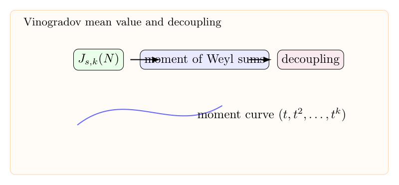
Now we discuss the discretization of decoupling type result. We could establish a relationship between the decoupling theorem and Vinogradov mean theorem. look at the sum:
This could be view as a norm of a constant function , with a lebergue measure on curve . this curve could be view as a canonical curve with non-vanish guess curvature.
this is very similar with the restriction theorem:
[restriction theorem]
let be $n-1$ dimension parabolic in , then guess curvature of is non-vanish. is a natural induced lebergue measure on , we have, for suitable exponents come from rescaling arument.
So it seems like these are the same thing, but unfortunately they are not,there are two things distinct them:
1.the density is defferent, it is a discrete sum in:
but a continue integral in:
so we need to construct a rescaling way to make the discretization one coverage to the continue one.a suitable fexiable function seems like
2.there
补充说明
以下是新整理的中文说明;上方旧博客原文保持不变。
Vinogradov mean value theorem 控制 Weyl sums 的高阶矩,是 Waring problem、指数和估计和 zeta 函数零点区域中的基础工具。Bourgain-Demeter-Guth 用 decoupling theorem 证明了主猜想。
Vinogradov mean value theorem 把 Weyl sums 的高阶矩与 moment curve decoupling 联系起来。
The technique that transform a problem which is in a linear setting to a multilinear setting is very powerful.
such like:
1.The renormalization technique in complex dynamic system, and the generalization
this is mainly the Ostrowoski representation,and something else.
2.Fouriour analysis
this can be view when it is difficult to investigate a quality about a function , it is always easier to take charge with some some part of , in this case is given by or like cut into a lot of small parts,deal with every part and use some inequality(always the triangle inequality or similar thing) to glue it into a whole estimate of the quantity of .
3.Multi-scales theory
this is used in the improve of Minkowski dimension of 3-dim kakeya set by Katz-Tao.
4.The proof of Bourgain-Sarnak-Ziegler theorem
Theorem(B-S-Z). Let with and let be a multiplicative function with . Let be a small parameter and assume that for all primes , , we have that for large enough
.
Then for N large enough
.
this theorem is not difficult to prove by bilinear method and Cauchy-Schwarz,you can see the detail in https://arxiv.org/abs/1110.0992v1.
According to this theorem,to get a good approximation of we use need a good approximation on .this will be much easier.but for the RHS is very complicated so I do not have a non-trivial estimate for until now.
5.The multiplier restriction theorem(Tao)
6.Some special construction in additive Combitriocs
Such like when we want to consider some set satisfied it is convenient to consider in a high dimensional linear space rather than in .
补充说明
以下是新整理的中文说明;上方旧博客原文保持不变。
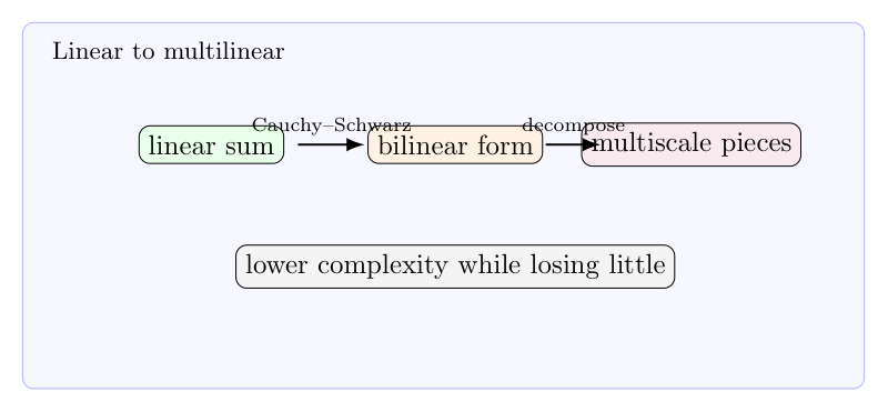
很多问题直接估计一个线性量很难,但把它平方、分解或转成多线性形式后,结构反而清楚。这就是从 linear 到 multilinear 的基本哲学。
从 linear 到 multilinear 的基本动作是用 Cauchy-Schwarz 或分解降低复杂度,同时保留主要信息。





 , where
  is a
is a  invariant measure.

 varies in all sequences of measure coverage to
  in the sense for all
  ,
,  measurable then
  .
. , shift map on countable alphabet.
 diffeomorphisms on compact manifold is asymptotically h-expensive.
 metric space
 is a continuous map.
 , then
  is still a metric.
 . This identity could be proved by the cretition of entropy by
  -seperate set and
  compact, for every ergodic measure
  .
. is the measure theoretic entropy of
  defined the moduli space of
  -invariant portability measure.
 defined the moduli space of ergodic
  satisfied simplified entropy formula if
  surfaced small and
  ,
,  .
. .
. suffciently small,
  ,
,  .
. .
. .
.  ,
,  ,
,  , satisfied:
 weakly.
 ,
, 
 .
. is a diffeomorphism and
  -invariant measure.
 is the multiplicity of
  and
and  .
. and
and  is equivalent to the Riemannian measure on
  diffemoephism, where
 is absolute continuous.
 have good regularity. But this idea is not complete to solve the problem.
 of
of  could be diagonal. Assume after diagonal the eigenvalue is
 .
. :
:
 ,
,  is the eigenvector space of
  . The dimension of $V_k$ is $dim V_k$.
 .
. is a measurable partition of
  , and we have:
 .
. . Estimate it is not very difficult. we need only observe the following two thing:
 exists a.e. in
  . and we product it and get :
 .
.


 .The graph is just like:
 .The graph is just like:


 .The graph is just like:
 .The graph is just like:
 .The graph is just like:
 . The graph of it is just like:
 and is just like 3 lines. And there are two singularity
  .
.


 :
:

 :
:


 is established. first
  by Otrokov,and later proved to be
  .
. , where A is a nonsingular 2*2 matrix. So we could classify the topological graph of the dynamic system.
 Every color in the graph is an area $P,Q$ do not have same component in it. And the boundary of areas is just the same component of
  if it exists.
 do not have same connected component then the intersection
  . And we can divide the space
  into finite parts,
  restrict to every part do not have the same component. And we have a upper bound control on the number of part when
  . A easy arrive bound could be
  .
. ,
,  are limit cycle and
  is inside of
  , then there is at least one singularity or another limit cycle contain in
  .
.
 . If the number of the limit cycle change, it must be the time to pass a singularity. and take
  , the dynamic system coverage to a very simlpe one and in particular it do not have limit cycle. So we need only look at the moments passing singularity.
 and
and  ,
,  ?
? , this amounts to the equation $latex \int_{\gamma_t}\frac{dz}{F(z)}=t$
 is the curve
  “truncated” at
  and the RHS is in particular **real**. This can be taken further, for example by assuming
  .
. -limit of a trajectory is either a point or a non-isolated cycle (center case).
 (*i.e.* a root of $F$) can only be of three types, according to the value of
  :
: .
. .
. petals:
  with multiplicity
  .
. ) with exactly
  separatrices, reaching the singularity in finite time. The bassins of attraction / center regions attached to the above singularities are delimited by the separatrices.
 . This started some works on the topic, for instance by Schub, Tischler, William (*The Newtonian graph of a complex polynomial*, 1988) or Benzinger (*Plane autonomous systems with rational vector fields*, 1991)…
 ) is associated to the separatrices, providing a complete conformal invariant.
 is called a Fatou coordinates. It is a rectifying chart for the vector field, and has many interesting dynamical properties.
 ). Is it classical ?
 .
. be the elementary symmetric polynomial in the eigenvalues of
  . For instance,
  is the trace and
  the determinant. The following formula gives
  whose entries are the scalar products
  .
.
 takes values in a subspace of dimension
  , which is the condition under which
  is a consequence of the identity
 , iff
, iff  arrive a minimum .
 make the Energy
  arrive a minimum.


 , and let
  be a compact set. Let
  denote the [[Lebesgue measure]] (volume) of
  by the ”’Minkowski–Steiner formula”’:

 , and:
 , so that:
 .
. -dimensional measure of the [[boundary (topology)|boundary]]
  of
of  ,
, are some [[continuous function]]s of
  (see [[quermassintegral]]s) and $\omega_{n}$ denotes the measure (volume) of the [[unit ball]] in
  :
: ,
, denotes the [[Gamma function]].
 gives the following well-known formula for the surface area of the [[sphere]] of radius
  ,
,  :
:
![= \lim_{\delta \to 0} \frac{[ (R + \delta)^{n} - R^{n} ] \omega_{n}}{\delta}](https://s0.wp.com/latex.php?latex=%3D+%5Clim_%7B%5Cdelta+%5Cto+0%7D+%5Cfrac%7B%5B+%28R+%2B+%5Cdelta%29%5E%7Bn%7D+-+R%5E%7Bn%7D+%5D+%5Comega_%7Bn%7D%7D%7B%5Cdelta%7D&bg=ffffff&fg=5e5e5e&s=0&c=20201002)
 ,
, is as above.
 .
. .
. with the Gromov-hausdorff metric on the space consist with convex open sets.
 points approximation in Gromov-hausdorff distance. and definitely carefully refinement of this kind of approximation could lead to the result of continuous of the energy
  it could be achieve with open convex set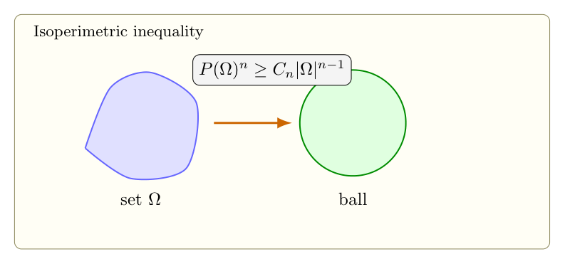
 (*)
(*) ,
,  . this is just the condition to make (*) be a elliptic equation.
 estimate and
  estimate in the inter. And the
  . then we can associate a measure
  ,and the following is right:
 ,
,  .
. coverage to
  coverage to
 ,
,  , then we have:

 is the Grassmannian of the d-dimensional vector subspaces of
  . For example,
 is the projective bundle of E. In the other direction, a Grassmann bundle is a special case of a (partial) flag bundle. Concretely, the Grassmann bundle can be constructed as a Quot scheme.
 .
. and
and is the determinant line bundle. Now, by the universal property of a projective bundle, the injection
 corresponds to the morphism over X:
 ,
, of
of  is given by[1]
 ,
, as the determination of transform:
  .
. as the average of determination of transform matrix of
  is equal to
  , i.e.:
 .
.
 ,
, .
.
 ?
? , then by following clear calculate:
![\int_{[0,1]^k}|f_k(x,N)|^{2s}dx_1...dx_k =\int_{[0,1]^k}|\sum_{1\leq n\leq N}e(nx_1+n^2x_2+...+n^kx_k)|^{2s}dx_1dx_2...dx_k &=\int_{[0,1]^k}\sum_{1\leq n_1,...,n_{2s}\leq N}e^{2\pi i[(n_1+...+n_{2s})x_1+...+(n_1^k+...+n_{2s}^k)x_k-(n_{s+1}+...+n_{2s})x_1-...-(n_{s+1}^k+...+n_{2s}^k)x_k]} &=|\{(n_1,...,n_{2s})| n_1^j+...+n_s^j=n_{s+1}^j+...+n_{2s}^j,\forall 1\leq j\leq k\}|](https://s0.wp.com/latex.php?latex=%5Cint_%7B%5B0%2C1%5D%5Ek%7D%7Cf_k%28x%2CN%29%7C%5E%7B2s%7Ddx_1...dx_k+%3D%5Cint_%7B%5B0%2C1%5D%5Ek%7D%7C%5Csum_%7B1%5Cleq+n%5Cleq+N%7De%28nx_1%2Bn%5E2x_2%2B...%2Bn%5Ekx_k%29%7C%5E%7B2s%7Ddx_1dx_2...dx_k+%26%3D%5Cint_%7B%5B0%2C1%5D%5Ek%7D%5Csum_%7B1%5Cleq+n_1%2C...%2Cn_%7B2s%7D%5Cleq+N%7De%5E%7B2%5Cpi+i%5B%28n_1%2B...%2Bn_%7B2s%7D%29x_1%2B...%2B%28n_1%5Ek%2B...%2Bn_%7B2s%7D%5Ek%29x_k-%28n_%7Bs%2B1%7D%2B...%2Bn_%7B2s%7D%29x_1-...-%28n_%7Bs%2B1%7D%5Ek%2B...%2Bn_%7B2s%7D%5Ek%29x_k%5D%7D+%26%3D%7C%5C%7B%28n_1%2C...%2Cn_%7B2s%7D%29%7C+n_1%5Ej%2B...%2Bn_s%5Ej%3Dn_%7Bs%2B1%7D%5Ej%2B...%2Bn_%7B2s%7D%5Ej%2C%5Cforall+1%5Cleq+j%5Cleq+k%5C%7D%7C+&bg=ffffff&fg=5e5e5e&s=0&c=20201002)
![J_{s,k}(N)=\int_{[0,1]^k}|f_k(x,N)|^{2s}dx_1...dx_k](https://s0.wp.com/latex.php?latex=J_%7Bs%2Ck%7D%28N%29%3D%5Cint_%7B%5B0%2C1%5D%5Ek%7D%7Cf_k%28x%2CN%29%7C%5E%7B2s%7Ddx_1...dx_k+&bg=ffffff&fg=5e5e5e&s=0&c=20201002)

![E_{[0,1]}(g)](https://s0.wp.com/latex.php?latex=E_%7B%5B0%2C1%5D%7D%28g%29&bg=ffffff&fg=5e5e5e&s=0&c=20201002) cut off $E_{[0,1]}(g)$ into a lot of small boxes
cut off $E_{[0,1]}(g)$ into a lot of small boxes  , then the $L_{d(d+1)})$ norms of the operator could be bounded very well, in fact it is near orthonagonal.
 ,$0<\delta\leq 1$. Then for each ball
  of radious at least
  .
.![||E_{[0,1]}g||_{L^{d(d+1)}(w_B)}<< \delta^{-\epsilon}(\sum_{J\subset [0,1],|J|=\delta}||E_Jg||^2_{L^{d(d+1)(w_B)}})^{\frac{1}{2}}](https://s0.wp.com/latex.php?latex=%7C%7CE_%7B%5B0%2C1%5D%7Dg%7C%7C_%7BL%5E%7Bd%28d%2B1%29%7D%28w_B%29%7D%3C%3C+%5Cdelta%5E%7B-%5Cepsilon%7D%28%5Csum_%7BJ%5Csubset+%5B0%2C1%5D%2C%7CJ%7C%3D%5Cdelta%7D%7C%7CE_Jg%7C%7C%5E2_%7BL%5E%7Bd%28d%2B1%29%28w_B%29%7D%7D%29%5E%7B%5Cfrac%7B1%7D%7B2%7D%7D&bg=ffffff&fg=5e5e5e&s=0&c=20201002)
 runs over a partition of
 ![[0,1]](https://s0.wp.com/latex.php?latex=%5B0%2C1%5D&bg=ffffff&fg=5e5e5e&s=0&c=20201002) in
in ![\int_{[0,1]^k}|\sum_{1\leq n\leq N}e(nx_1+n^2x_2+...+n^kx_k)|^{2s}dx_1dx_2...dx_n](https://s0.wp.com/latex.php?latex=%5Cint_%7B%5B0%2C1%5D%5Ek%7D%7C%5Csum_%7B1%5Cleq+n%5Cleq+N%7De%28nx_1%2Bn%5E2x_2%2B...%2Bn%5Ekx_k%29%7C%5E%7B2s%7Ddx_1dx_2...dx_n&bg=ffffff&fg=5e5e5e&s=0&c=20201002)
 norm of a constant function
  , with a lebergue measure
  on curve
  . this curve
 , then guess curvature of
  is a natural induced lebergue measure on
  come from rescaling arument.


 or
or  like cut
  with
with  and let
  be a multiplicative function with
  . Let
. Let  be a small parameter and assume that for all primes
  ,
,  , we have that for
  .
. .
. we use need a good approximation on
  .this will be much easier.but for the RHS
  is very complicated so I do not have a non-trivial estimate for
  satisfied
  it is convenient to consider in a high dimensional linear space
  rather than in
  .
.