In this note we discuss the Schauder theory for uniformly elliptic linear equations and Sobelov inequality.
the three main topics ars a priori estimate in Holder norms,regularity of arbitrary solutions and the solvability of the Dirichlet problem.Among these topics,a priori estimates are the most fundamental and the basis of the follows two.we will discuss both the interior Schauder estimate and global Schauder estimate.
-Schauder Theory-
1. Interior Schauder Theory
be a domain in ,bounded most of the time. be defined in ,with .where .
we consider the operator given by,
easy to see is defined for any .
the operator is always be assumed to be strictly elliptic in ;namely,
for any ,where is a positive constant.
1.1. Interior Schauder Estimate
define the weighted norm,
easy to see come from a scaling.
consider the PDE.
we want to proof this type estimate,
where
we first deal with a easy case, is constant. in this case we proof the estimate:
Lemma 1 ,for some ,and be a constant symmetric matrix satisfying
. suppose satisfies:
then ,,moreover,
Proof: to continue,we prove an interpolation inequality for Holder continuous functions.
Lemma 2 Let and be a ball of radius in ,then, (1)for any ,
(2)for any ,
(3)for any ,
where is a positive constant depending on n and .
Proof:
Corollary 3 Let and be a ball of radius in .Then,for any ,
Proof:
Now we are ready to prove an interior estimate for -norms of solutions of uniformly elliptic equations.The trick is to freeze coefficients.
Lemma 4 2. Global Schauder Theory
-Sobelov inequality-
Theorem 5
moreover,we have: , ,
Proof:
suffice to proof:
obvious we have:
so .
so
use the similar argument as to prove the situation .
suffice to prove .
obvious we have:. . Q.E.D.
4.
moreover,we have: , ,
,
then is well-defined by the following lemma:
Lemma 6 continously for any q, satisfy .
furthermore,for any
Proof: directly calculate follows that :
now follows young inequality and this priori estimate we have:
and by the priori estimate,we have:
Q.E.D.
Lemma 7 ,. constant depend only on ,such that
Proof: we have
then take suffice large. Q.E.D.
Lemma 8 let
a.e. in .
Proof: frist zero extended to whole space.and we have .
forall ,so
Q.E.D.
Theorem 9 let ,then there exists constant such that
The given “smooth” initial : T small ,,the solution exists on
equation is possible system.
Deturk Trick
“Threshold type theorem”
Ricci flow:
Mean curvature flow:
HMF:
Calabi flow:
pf of observation 4:if threshold condition hold for ,then we can bound ang norm of solution.
“geometry”
2. smooth manifold with conical singularities
on surface we can define conical singularity.
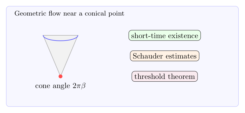
Definition 1 (conical singularity) ,,where ,the angle of conical singularity is .
iff conical background metric : near p,, is the interpolation coordinate chart.
it is easy to chake the form is independent with the coordinate chart ,so the definition is well defined.
3. rough line of proof
initial ,
Step 1:(Short time existence)
state and proof the “magic theorem”:
1.we need to explain what is smooth,to define a Banach space ,maybe type.
2.to proof the “magic theorem” under the setting.maybe use shauder fix point theorem or contraction map theorem or else.
3.so the problem reduce to get this type estimate,
if .
define . is continuous, is convex, is a pre-compact set.for suffice small
the difficult is to set up the continuous of operator
Schauder estimate tell us:
this give us some useful information to construct space .
Step 2:(Threshold type theorem,long time existence)
Threshold as long as is bounded.
This type theorem is relate to the maximal internal in which solution existence is closed.
Basically is based on Alzalo-Ascoli theorem.
Step3:(More regularity) 1.the question does not existence for smooth manifold.(why)
2.singular space. small space small space.
what is the optimal regularity?
the problem naturally come from both “pure PDE” and “application for geometry problem”.
where f is a function with nice regularity.
Functional analysis:
extension to:
which is a self-adjoint extension.and then use the theory of operator semi-group.the problem can be solved.
remark:the extension is not unique so the information we know for the solution is very little.and because the really true extension which is suit for our geometry setting is just one extension.so the treat of Functional analysis is not enough for us.
Elementary treat:
consider the simplest case,smooth manifold with only one singularity.
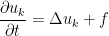
we set is the manifold cut off form with a boundary more and more near the singularity. consider the equation on each ,i.e.:
on
with boundary condition:
Drichlet condition
or Neumann condition
we choose Neumann condition there and at last we will see the solution come from Dirichlet condition is the same with the solution come from Neumann condition.
Under the general setting this become:
when , do we have ?
we need priori estimate: Schauder estimate for serious parabolic equation tell us:
for equation on with priori estimate , we have:
wher is the maximal such that geodesic ball .
For general setting :
we know
this is what Schauder estimate tell us.
1.the uniform estimate with k: independent of k.(now we do not know what the norm need to be)
we have estimate and the energy estimate as follows:
from maximal principle,easy to get norm estimate.
the point is the equation is strict parabolic so we have strong maximal principle and to construct suit bump function we can estimate norm of .
from energy method we can estimate .
the point is: .
so we get:
so we can bounded .
for the general case:the equation becomes:
but there is a hide Dragon,we need the condition .
otherwise we will get solution .
but in this case we still have the two necessary estimate(esay to see the above argument still make sense).
in this case to prove the short time existence we need follow four claims is ture.
as
as
as
as
5. Construct the suitable Banach space
call the space construct follow the Mixed-Holder-Sobolev space for simply case,consider smooth manifold with only one conical singularity.
first cover the whole manifold by a open set have positive distance t=with the conical singularity and a countable group of set ,which is balls center at singularity with radius .(where )
i.e.
Definition 2 ()
easy to see the definition is independent with the cover and the local interpolation coordinate chart.
one thing is also trivial,is that we have the schauder estimate under the norm .
that is
on . on . then
in fact we only need to add each inequality come from each open set of the cover by Schauder estimate to proof this.
on the other hand we need a suitable Sobolev type norm.
Definition 3 ()
Definition 4 () the set of all f in with finite ,
in Banach space.
Assume norm on
Definition 5 (]
\end) from the definition,easy to see
om
easy from the classical schauder estimate.
Definition 6 ()
Key point:
Definition 7 (] is the set of in with finite
\end) 6. What is a solution of equation
trivial sense:
satisfied equation point-wise on .
weak sense:
1.trivial case
2.
1. rough outline of heat kernel proof of Atiyah-singer index theorem
1.1. proof strategy
Theorem 1 (Mckean-Singer formula.)
from this we know Fredholm operator deformation invariance,in the same time we need chern-weil theory.
Main challenge:
1. in the expansion on heat kernel ,we need to proof when , the limit exist and find a way to calculate it.
2. indentify the limit as .
Proof: Our proof road锛� mckean-singer formula local-index thm A-S index thm Riemann-roch-Hirzebunch theorem.
1.2. preliminary work
superbundle: .
on compact manifold , is a self-adjoint operator . . .
observe that: is symmetric eigenvalue space of is finite dimention in particular is finite dimesion is finite dimension.
dimention of superspace :
Def: .
Lemma:
1.Let be a self-adjoint Dirac operator on a clifford module over a compact manifold ,then
in particular,
where coker .
2.Let be a differential operator acting on a -graded vector bundle ,then .
the proof of this two lemma is easy,leave sas exercise.
1.3. Mckean-Singer formula
the formula is:
the expression of heat operator by spectral measure is:
proof 1:
we have first eigenvalue estimate on compact manifold:
on the other hand ,we need to show is independent with ,in fact:
odd parity : . supercommunater
q.e.d
proof2:
by spectral decompositon of :
observe that: for . . (detail in [BGV])
q.e.d
Corallary: the index of a smooth on-parameter family of Dirac operator is constant.
what we have proved is:
1.4. analytic formula of ind
from the discuss of heat kernel in section 2,we know following result(section 2 only discuss the case of function but use the similar way we can get similar result on bundle):
on the other hand: .
and use the Mckean-Singer formula,we get: ind (D^+)&=&Str(e^{-tD^2})
&=&Tr(e^{-tD^+D^-})-Tr(e^{-tD^=D^-})
&=&\int\limits_M Tr(K_t(x,y,D^-D^+)) – \int\limits_M Tr(k_t(x,y,D^+D^-))
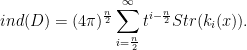
&=&\sum\limits_{i=0}^{\infty} t^{i-\frac{n}{2}}a_i(D^+D^-) – \sum\limits_{i=0}^{\infty} t^{i – \frac{n}{2}}a_i(D^+D^-). where is the heat trace invariants.
take ,the only thing make sense is the series of order ,and we want to proof:
But the difficult thing is that the high order series is very hard ro calculate….
our strategy is following:
Step1: proof has a limit as i.e index density.
step2:use a rescaling of space,time,clifford bundles ,to find a way that make us only need to calculate the leader coefficient.
1.5. From the McKean鈥揝inger formula to the index theorem
Let be a compact oriented Riemannian manifold of even dimension . We will write for the heat kernel associated to . The diagonal is a section of which is iso- morphic to . Using this isomorphism, we define a filtration on , induced by the filtration on . Elements of are given 0-degree. Denote by the subbundle of consisting of all elements of degree less or equal to .
the following theorem hold:
Theorem 1. The following statements hold:
1. The coefficients have degree less or equal to . In other words, . 2. If ,where denotes the restriction of the symbol map, then:
the important observation is that the of order less than n all vanish,in the other word:
lemma2:for any quadratic space of dimension ,.
Proof: Let be a basis of . For any multi-index , denote by the Clifford product .Then the set is a basis for .If,there is at least one such that , and we have
q.e.d
so take , we get:
now we want to identify the term as a characteristic form on :
Lemma 3. Let be a Euclidean space. There is, up to a constant factor, a unique supertrace on , equal to where denotes the symbol map and is the projection of onto the coefficient of if form an oriented orthonormal basis of . Furthermore, the supertrace defined above equals:
rmk:(The map is also called the canonical Berezin integral.)
proof:
the dimension of space is one because of and it never be empty because there is a natural defined supertrace on .so the only thing we need to do is to determine the constant,in face we only need to calculate the supertarce on any non-zero element .for instance the chirality operator . We have that and therefore for all .
q.e.d
so we know: section :
theorem1 implies then the following theorem for the index of a Dirac operator associated to a Clifford connection which is known as the local index theorem.
Theorem 2. (Local index theorem) Let be a compact, oriented even-dimensional manifold and let be a Clifford module with Clifford connection . Let be the associated Dirac operator. Then exists and is obtained by taking the -th form piece of
rmk:This theorem only holds for Dirac operators associated to Clifford connections, which are those which are compatible with the Clifford action. However, since the index of a Dirac operator is independent of the Clifford superconnection used to define it, we get Atiyah鈥揝inger index formula for any Dirac operator.
Theorem 3. (Atiyah鈥揝inger Index Theorem) Let be a compact, oriented, even-dimensional manifold and let be a Dirac operator on a Clifford module . Then the index of is given by :
hence theorem 3 is a consequence of theorem 1.
up to now,to prove index theorem ,we only need to prove theorem 1.
1.6. idea of the proof of theorem 1
we give the clear proof in appendix锛宼here we explain the idea:
To prove Theorem 4.11 we mainly follow Chapter 4 of [BGV] but rearrange the different steps in order to make the proof clearer, at least for us. Let us summarize the first part of the proof:
1. The idea of the proof is to work in normal coordinates around a point . Near the diagonal, we use parallel transport to pull back the heat kernel which is a section of the vector bundle and define a new kernel , a section of for some twisting space . Using the symbol isomorphism , we can look at as a section of .
2. We use Lichnerowicz鈥� formula to get the explicit form of the operator such that the kernel satisfies the heat equation .
3. In a third step, we define a rescaling of space, time and the Clifford algebra, introduced by Getzler. This rescaling has the effect that the leading coefficient of the asymptotic expansion of the rescaled kernel is exactly the differential form of theorem 1 which leads to a reformulation of Theorem 1.
\appendix
2. Chern-Weil theory
some text in Appendix A
3. Complete proof of theorem 1
some text in Appendix B
补充说明
以下是新整理的中文说明;上方旧博客原文保持不变。
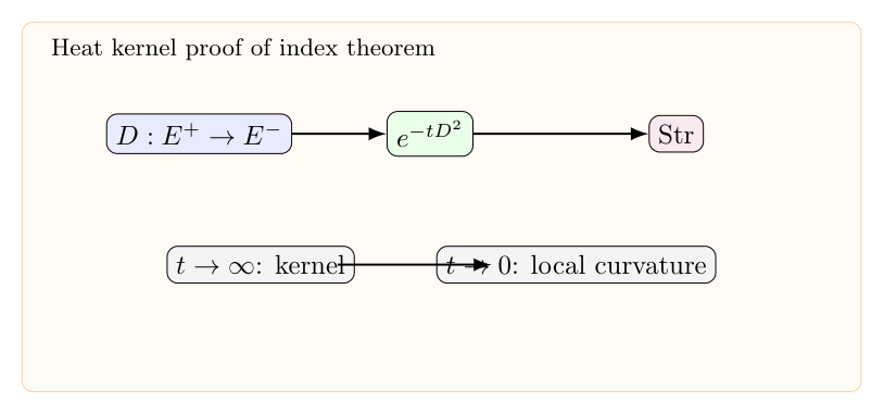
热核证明指标定理的主线可以压缩成一句话:McKean-Singer 公式把 index 写成 heat operator 的 supertrace;再让 $t\to0$,用热核局部展开读出曲率多项式。
McKean-Singer 公式让 index 等于 heat operator 的 supertrace,小时间极限给出局部指标密度。
campact,complete,Riemann manifold without boundary,dim . is the Levi-civita connection on ,. genus form:
by chern-weil theory,we know: is closed. is exact.
so we can def is a metric on M.
1.2. dirac bundle
is a dirac bundle. is dirac operator. the twisting curvature of .
1.3. supertrace
. induce map:
determined by:
1.4. chern class
by chern-weil theory,we know:
1. closed form.
2. only depend on the topology of E.
Whitney product formula.
1.5. Atiyah-singer index theorem
2. heat kernel
2.1. basic setting
Assume M is a general Riemann manifold ,assume
Where .
complete with the norm is the sobolev space .
The extension of operator in is called ,assume is restrict on , extend to called , is complete with the norm , of course .
Sobelev theory tell us, if is a complete Riemann manifold,then .
Operator ,satisfied ,where * is the Hodge-star operator , is the 1-form, iff one of is compact supp.
By a lemma from Gaffney (Ann. of Math , 60,1954,458-466) we have .
the laplace operator(with Direchlet boundary condition or Neumann boundary condition) is , When M is with smooth boundary,then ,assume M is complete (),then because ,Gaffney proved(Ann. of Math , 60 ,1954,140-145),
.
As we all known, is self-adjoint operator,so make up a bounded self-adjoint operator semi group,by the self-adjoint operator theory,if is the spectrum measure of ,then
.
And for ,.when ,
where is basic on Weyl theory.
2.2. existence of heat kernel
Now we proof the basic fact: : assume is a complete manifold,then there exist a heat kernel ,and ,,satisfied:
Proof:
(A) first proof, .to proof this,we first proof,in weak sense:
in fact,we have:
rmk: the limit is take in the space,every step in the caculate make sence because of the dominating convergence theorem.
so what have we proved ,in fact we proved in the classical sence, exist. and our strategy is to proof any order of weak derivatives of it exist and then use the embedding theorem to prove it is smooth.
in fact to proof (in weak sence),we need only to proof: we have:
but because of ,this is obvious,and similar we can proof that (in the weak sence):
rmk: there is some thing to explain,why .
anyway,we observe that is the laplace operator on .and we have proved ,and we know that .so we proved
and now we easy to observe that,
if ,then:
.
so
.
Rmk:,so derivatives is in classical sense.
(B) to proof .
by the decomposition of unity,we can assume ,and sufficed small.
consider the operator and its quasi fundamental solution (paramatrix) see next section for the serious definition ,
. and ,and when suffice small,,we have expansion:
where Riemann distance.,for ,
use instead of ,and assume ,
assume ,then
this is because ,when ,so ,so .because:
so and have the same expansion .because so ,we have:
the equality arrive is because of the prop of .
on the other hand ,by the definition of ,we can check:
when is fix and ,, so
we call is the kernel of .
for prop (1), is from the operator is self-adjoint,prop (2) is just .
now we proof prop (3),by definition:
and we know so.
proof prop (4),by and wo know:
QED.
rmk: for the manifold with bounded,we can also proof the existence of heat kernel with Dirchlet or Neumann boundary condition.(L.Chavel. Eigenvalues in Riemannian Geometry,Academic Press,1984)
2.3. quasi fundamental solution of heat equation
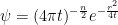
it is well known that for , the fundamental solution of heat equation is .
for general Riemann manifold ,we want to find the fundamental solution of heat equation with this form:
where is the Riemann distance of two point of M. take the normal coordinate around point , .(the length of geodesic connect ).
it is well known that there exist functions only depend on :
take:
and
then
because of
we know:
problem become to solve the equations:
which is equivalent to:
solve it:
so . and:
take the cut function,:
take:
of course:
this is to say: is the quasi fundamental solution of heat equation. from the equation:
we know if has suffise high zero ,then so is the solution of heat equation,so can approximate heat equation to any order.
2.4. basic proposition of heat kernel
:
proof strategy : begin with expansion of heat kernel and integral on a geodesic sphere and take the radius ,use the stokes formula and maximal value principle to proof is always positive.
: assume is a constant curvature complete riemann manifold (space form),then only depends on ,and. proof is similar to .
(heat kernel comparision theorem,Cheeger-Yau).:
assume is a complete riemann manifold ,,, heat kernel of and heat kernel of geodesic ball in space form satisfied:
(bounded condition is Derichlet condition or Neumann condition).
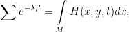
proof strategy: basically we use the formula .and the two lemma. : assume is a compact reimann manifold , is a orthonormal basis of special function on , is the corresponding spectrum,then the fundamental solution (heat kernel) has the expansion:
Basic setting:
Let be a compact Riemannian manifold of dimension , let be an – normalized eigenfunction of the Laplacian:
latex N \phi_{\lambda} =\{x:\phi_{\lambda}(x)=0\}$
be its nodal hypersurface. Let denote its -dimensional Riemannian hypersurface measure. In this note we prove:
Theorem:
for and metric ,there exists a constant so that:
A crucial identity:
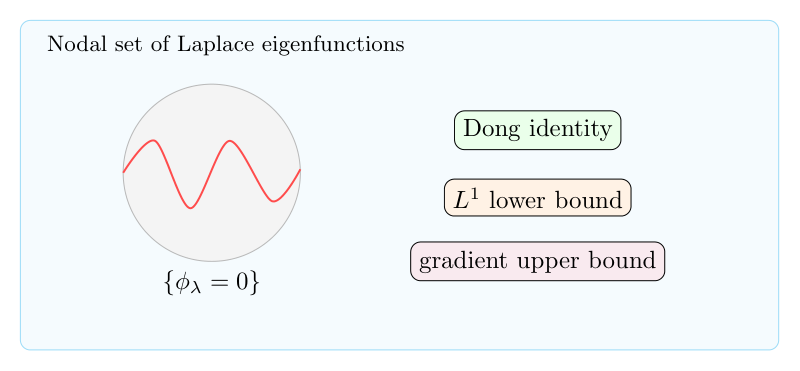
proof of theorem 1 is based on following identity:
theorem:
for any smooth Riemannn manifold ,we have,
moreover,,
Proof:
observed we have that,
on ,use divergence theorem:
\begin{eqnarray*}
\int_M(\Delta+\lambda^2)f \phi_{\lambda} dV&=&\int_M(\Delta+\lambda^2)\phi_{\lambda}f dV+\int_{\partial M} -g(\upsilon,\phi_{\lambda}\nabla f)dS+\int_{\partial M} g(\upsilon,f\nabla\phi_{\lambda})dS\\
&=&\int_{\partial M} g(\upsilon,f\nabla\phi_{\lambda}) \\
&=&\int_{\partial M} f\phi_{\lambda}dS
\end{eqnarray*}
the same identity is true on
so we have:
Estimate hausdorff measure of nodal sets:
take in theorem 2,we have:
so to get estimate hausdorff measure of nodal sets,we need to estimate: ,$||\nabla\phi_{\lambda}||_{\infty}$ ,this two guys are easy to get good estumate….and we will get a lower bound estimate of measure of nodal set:
Estimate: , :
normalized norm of
:
we have a yau types gradients estimate
Estimate upper bound of measure:
to get upper bound estimate,from identity we need to estimate:,,and we will get:
\section{Birkhoff回复定理蕴含Van Der Warden定理}
\subsection{Van Der Warden定理与它的动力系统解释}
这是一个组合定理,原始证明是很trick的,单遵老先生有一个证明,很trick,高中的时候尝试过证明,自己证了一个星期证明不出来就看掉了,现在回想起来应该跟当时的工具太原始了有关系。我想强调的是并不是数学思想的飞跃,而是数学工具的升级使得这个问题变简单了。\\





![I=I_{0,0}=[0,1]](https://s0.wp.com/latex.php?latex=I%3DI_%7B0%2C0%7D%3D%5B0%2C1%5D&bg=ffffff&fg=5e5e5e&s=0&c=20201002)


![I_{n,j}=[j2^{-n},(j+1)2^{-n}]](https://s0.wp.com/latex.php?latex=I_%7Bn%2Cj%7D%3D%5Bj2%5E%7B-n%7D%2C%28j%2B1%292%5E%7B-n%7D%5D&bg=ffffff&fg=5e5e5e&s=0&c=20201002)





 be a domain in
  ,bounded most of the time.
 be defined in
  .where
  .
. given by,
 is defined for any
  .
.
 ,where
  is a positive constant.
 norm,
norm,![\displaystyle |u|^*_{C^{k,\alpha}(B_R)}=\sum_{i=0}^k R^i|D^iu|_{L^{\infty}(B_R)}+R^{k+\alpha}[D^ku]_{C^{\alpha}(B_R)}](https://s0.wp.com/latex.php?latex=%5Cdisplaystyle+%7Cu%7C%5E%2A_%7BC%5E%7Bk%2C%5Calpha%7D%28B_R%29%7D%3D%5Csum_%7Bi%3D0%7D%5Ek+R%5Ei%7CD%5Eiu%7C_%7BL%5E%7B%5Cinfty%7D%28B_R%29%7D%2BR%5E%7Bk%2B%5Calpha%7D%5BD%5Eku%5D_%7BC%5E%7B%5Calpha%7D%28B_R%29%7D&bg=ffffff&fg=000000&s=0&c=20201002)
 come from a scaling.


 is constant. in this case we proof the estimate:
 ,for some
  ,and
,and  be a constant symmetric
  matrix satisfying
 . suppose
  satisfies:
 ,moreover,
![\displaystyle |u|^*_{C^{2,\alpha}(B_{\frac{R}{2}})}\leq C[|u|_{L^{\infty}(B_R)}+R^2|f|^*_{C^{\alpha}(B_R)}]](https://s0.wp.com/latex.php?latex=%5Cdisplaystyle+%7Cu%7C%5E%2A_%7BC%5E%7B2%2C%5Calpha%7D%28B_%7B%5Cfrac%7BR%7D%7B2%7D%7D%29%7D%5Cleq+C%5B%7Cu%7C_%7BL%5E%7B%5Cinfty%7D%28B_R%29%7D%2BR%5E2%7Cf%7C%5E%2A_%7BC%5E%7B%5Calpha%7D%28B_R%29%7D%5D&bg=ffffff&fg=000000&s=0&c=20201002)
 to continue,we prove an interpolation inequality for Holder continuous functions.
 and
and  be a ball of radius
  ,
,![\displaystyle \mu^{\alpha}R^{\alpha}[u]_{C^{\alpha}(B_R)}\leq C[\mu R |\nabla u|_{L^{\infty}(B_R)}+|u|_{L^{\infty}(B_1)}]](https://s0.wp.com/latex.php?latex=%5Cdisplaystyle+%5Cmu%5E%7B%5Calpha%7DR%5E%7B%5Calpha%7D%5Bu%5D_%7BC%5E%7B%5Calpha%7D%28B_R%29%7D%5Cleq+C%5B%5Cmu+R+%7C%5Cnabla+u%7C_%7BL%5E%7B%5Cinfty%7D%28B_R%29%7D%2B%7Cu%7C_%7BL%5E%7B%5Cinfty%7D%28B_1%29%7D%5D&bg=ffffff&fg=000000&s=0&c=20201002)
![\displaystyle \mu R |\nabla u|_{L^{\infty}(B_R)} \leq C[\mu^{1+\alpha}R^{1+\alpha}|\nabla u|_{C^{\alpha}(B_R)}+|u|_{L^{\infty}(B_1)}]](https://s0.wp.com/latex.php?latex=%5Cdisplaystyle+%5Cmu+R+%7C%5Cnabla+u%7C_%7BL%5E%7B%5Cinfty%7D%28B_R%29%7D+%5Cleq+C%5B%5Cmu%5E%7B1%2B%5Calpha%7DR%5E%7B1%2B%5Calpha%7D%7C%5Cnabla+u%7C_%7BC%5E%7B%5Calpha%7D%28B_R%29%7D%2B%7Cu%7C_%7BL%5E%7B%5Cinfty%7D%28B_1%29%7D%5D&bg=ffffff&fg=000000&s=0&c=20201002)
 ,
,![\displaystyle \mu R|\nabla u|_{L^{\infty}(B_R)}\leq C[\mu^2R^2|\nabla^2 u|_{L^{\infty}(B_R)}+|u|_{L^{\infty}(B_R)}]](https://s0.wp.com/latex.php?latex=%5Cdisplaystyle+%5Cmu+R%7C%5Cnabla+u%7C_%7BL%5E%7B%5Cinfty%7D%28B_R%29%7D%5Cleq+C%5B%5Cmu%5E2R%5E2%7C%5Cnabla%5E2+u%7C_%7BL%5E%7B%5Cinfty%7D%28B_R%29%7D%2B%7Cu%7C_%7BL%5E%7B%5Cinfty%7D%28B_R%29%7D%5D+&bg=ffffff&fg=000000&s=0&c=20201002)
 is a positive constant depending on n and
  .
. and
and  ,
,![\displaystyle \sum_{i=0}^2(\mu R)^i|\nabla^i u|_{L^{\infty}(B_R)}+\sum_{i=0}^1(\mu R)^{i+\alpha}[\nabla^i u]_{C^{\alpha}(B_R)}\leq C[(\mu R)^{2+\alpha}[\nabla^2 u]_{C^{\alpha}(B_R)}+|u|_{L^{\infty}(B_R)}]](https://s0.wp.com/latex.php?latex=%5Cdisplaystyle+%5Csum_%7Bi%3D0%7D%5E2%28%5Cmu+R%29%5Ei%7C%5Cnabla%5Ei+u%7C_%7BL%5E%7B%5Cinfty%7D%28B_R%29%7D%2B%5Csum_%7Bi%3D0%7D%5E1%28%5Cmu+R%29%5E%7Bi%2B%5Calpha%7D%5B%5Cnabla%5Ei+u%5D_%7BC%5E%7B%5Calpha%7D%28B_R%29%7D%5Cleq+C%5B%28%5Cmu+R%29%5E%7B2%2B%5Calpha%7D%5B%5Cnabla%5E2+u%5D_%7BC%5E%7B%5Calpha%7D%28B_R%29%7D%2B%7Cu%7C_%7BL%5E%7B%5Cinfty%7D%28B_R%29%7D%5D&bg=ffffff&fg=000000&s=0&c=20201002)
 -norms of solutions of uniformly elliptic equations.The trick is to freeze coefficients.
 ,
,  ,
,



 .
.

 to prove the situation
  .
. .
. .
.



![{\leq \frac{c}{n}\sum_{i=1}^n\tilde C p[(\int_{\Omega} (|u|^{p-1})^{\frac{p}{p-1}})^{\frac{p-1}{p}}+(\int_{\Omega} |D_iu|^p)^{\frac{1}{p}}]^{\frac{1}{p}} }](https://s0.wp.com/latex.php?latex=%7B%5Cleq+%5Cfrac%7Bc%7D%7Bn%7D%5Csum_%7Bi%3D1%7D%5En%5Ctilde+C+p%5B%28%5Cint_%7B%5COmega%7D+%28%7Cu%7C%5E%7Bp-1%7D%29%5E%7B%5Cfrac%7Bp%7D%7Bp-1%7D%7D%29%5E%7B%5Cfrac%7Bp-1%7D%7Bp%7D%7D%2B%28%5Cint_%7B%5COmega%7D+%7CD_iu%7C%5Ep%29%5E%7B%5Cfrac%7B1%7D%7Bp%7D%7D%5D%5E%7B%5Cfrac%7B1%7D%7Bp%7D%7D+%7D&bg=ffffff&fg=000000&s=0&c=20201002)
 . Q.E.D.

![{\mu\in (0,1]}](https://s0.wp.com/latex.php?latex=%7B%5Cmu%5Cin+%280%2C1%5D%7D&bg=ffffff&fg=000000&s=0&c=20201002) ,
,
 is well-defined by the following lemma:
 continously for any q,
 satisfy
  .
.

 directly calculate follows that :





 .
. constant depend only on
  ,such that
![\displaystyle \int_{\Omega} exp[\frac{g}{c_1||f||_p}]^{p^`}dx\leq c_2|\Omega|,p^`=\frac{p}{p-1}](https://s0.wp.com/latex.php?latex=%5Cdisplaystyle+%5Cint_%7B%5COmega%7D+exp%5B%5Cfrac%7Bg%7D%7Bc_1%7C%7Cf%7C%7C_p%7D%5D%5E%7Bp%5E%60%7Ddx%5Cleq+c_2%7C%5COmega%7C%2Cp%5E%60%3D%5Cfrac%7Bp%7D%7Bp-1%7D&bg=ffffff&fg=000000&s=0&c=20201002)


 suffice large. Q.E.D.

 to whole space.and we have
  .
.
 ,so
,so
 ,then there exists constant
 ![\displaystyle \int_{\Omega}exp[\frac{|u|}{c_1||Du||_n}]^{\frac{n}{n-1}}dx\leq c_2|\Omega|](https://s0.wp.com/latex.php?latex=%5Cdisplaystyle+%5Cint_%7B%5COmega%7Dexp%5B%5Cfrac%7B%7Cu%7C%7D%7Bc_1%7C%7CDu%7C%7C_n%7D%5D%5E%7B%5Cfrac%7Bn%7D%7Bn-1%7D%7Ddx%5Cleq+c_2%7C%5COmega%7C&bg=ffffff&fg=000000&s=0&c=20201002)
 ,then
,then  ,
, .
.

 ,
, ,
,


 T small ,
 ,the solution exists on
 ![{[0,T]}](https://s0.wp.com/latex.php?latex=%7B%5B0%2CT%5D%7D&bg=ffffff&fg=000000&s=0&c=20201002)
 norm of solution.
 ,
, ,where
  ,the angle of conical singularity
  is
is  .
. :
:  ,
, is the interpolation coordinate chart.
 ,
,
 ,maybe
  type.
type. .
.![{T_{[0,T]}:A(\Omega \times [0,T]) \longrightarrow A(\Omega \times [0,T])}](https://s0.wp.com/latex.php?latex=%7BT_%7B%5B0%2CT%5D%7D%3AA%28%5COmega+%5Ctimes+%5B0%2CT%5D%29+%5Clongrightarrow+A%28%5COmega+%5Ctimes+%5B0%2CT%5D%29%7D&bg=ffffff&fg=000000&s=0&c=20201002) .
. ![{T_{[0,T]}}](https://s0.wp.com/latex.php?latex=%7BT_%7B%5B0%2CT%5D%7D%7D&bg=ffffff&fg=000000&s=0&c=20201002) is continuous,
is continuous,![{Dom(T_{[0,T]})}](https://s0.wp.com/latex.php?latex=%7BDom%28T_%7B%5B0%2CT%5D%7D%29%7D&bg=ffffff&fg=000000&s=0&c=20201002) is convex,
is convex,![{Im(T_{[0,T]})}](https://s0.wp.com/latex.php?latex=%7BIm%28T_%7B%5B0%2CT%5D%7D%29%7D&bg=ffffff&fg=000000&s=0&c=20201002) is a pre-compact set.for
is a pre-compact set.for 
 is bounded.
 small space
  small space.


 is the manifold cut off form
  with a boundary more and more near the singularity. consider the equation on each


 , do we have
  ?
? on
on  , we have:
 is the maximal such that geodesic ball
  .
.


 independent of k.(now we do not know what the norm
  need to be)
 estimate and the energy estimate as follows:
 is strict parabolic so we have strong maximal principle and to construct suit bump function we can estimate
  .
. .
.


![{=-2[\int_{M_k}|\frac{\partial}{\partial t}u_k|^2-\int_{M_k} f\cdot \frac{\partial}{\partial t}u_k]}](https://s0.wp.com/latex.php?latex=%7B%3D-2%5B%5Cint_%7BM_k%7D%7C%5Cfrac%7B%5Cpartial%7D%7B%5Cpartial+t%7Du_k%7C%5E2-%5Cint_%7BM_k%7D+f%5Ccdot+%5Cfrac%7B%5Cpartial%7D%7B%5Cpartial+t%7Du_k%5D%7D&bg=ffffff&fg=000000&s=0&c=20201002)


 .
.
 .
.


 .
. .
.


 ,which is balls center at singularity
  with radius
  .(where
  )
)
 )
)

 .
.  on
on  . then
 )
)
 ) the set of all f in
  with finite
  ,
,
![{C^{k,\alpha}(B\times [o,T])}](https://s0.wp.com/latex.php?latex=%7BC%5E%7Bk%2C%5Calpha%7D%28B%5Ctimes+%5Bo%2CT%5D%29%7D&bg=ffffff&fg=000000&s=0&c=20201002) on
on ![{B\times [0,T]}](https://s0.wp.com/latex.php?latex=%7BB%5Ctimes+%5B0%2CT%5D%7D&bg=ffffff&fg=000000&s=0&c=20201002)
 ]
]![{f: S\times [0,T] \longrightarrow R }](https://s0.wp.com/latex.php?latex=%7Bf%3A+S%5Ctimes+%5B0%2CT%5D+%5Clongrightarrow+R+%7D&bg=ffffff&fg=000000&s=0&c=20201002)
![\displaystyle ||f||_{\rho^{l,\alpha,[0,T]}}=sup_{k=0,1,2,...,\infty}||f(2^{-k}\rho,\theta,4^{-k}t)||_{C^{l,\alpha}((B_1-B_{\frac{1}{2}})\times [0,4^{-k}T])}+||f||_{C^{l,\alpha}(U\times[0,T])}](https://s0.wp.com/latex.php?latex=%5Cdisplaystyle+%7C%7Cf%7C%7C_%7B%5Crho%5E%7Bl%2C%5Calpha%2C%5B0%2CT%5D%7D%7D%3Dsup_%7Bk%3D0%2C1%2C2%2C...%2C%5Cinfty%7D%7C%7Cf%282%5E%7B-k%7D%5Crho%2C%5Ctheta%2C4%5E%7B-k%7Dt%29%7C%7C_%7BC%5E%7Bl%2C%5Calpha%7D%28%28B_1-B_%7B%5Cfrac%7B1%7D%7B2%7D%7D%29%5Ctimes+%5B0%2C4%5E%7B-k%7DT%5D%29%7D%2B%7C%7Cf%7C%7C_%7BC%5E%7Bl%2C%5Calpha%7D%28U%5Ctimes%5B0%2CT%5D%29%7D&bg=ffffff&fg=000000&s=0&c=20201002)


![\displaystyle ||u||_{\rho^{l+2,\alpha,[0,T]}}\leq C(||u_0||_{\varepsilon^{l,\alpha}}+||f||_{\rho^{l,\alpha,[0,T]}}+||u||_{C^0(S\times [0,t])})](https://s0.wp.com/latex.php?latex=%5Cdisplaystyle+%7C%7Cu%7C%7C_%7B%5Crho%5E%7Bl%2B2%2C%5Calpha%2C%5B0%2CT%5D%7D%7D%5Cleq+C%28%7C%7Cu_0%7C%7C_%7B%5Cvarepsilon%5E%7Bl%2C%5Calpha%7D%7D%2B%7C%7Cf%7C%7C_%7B%5Crho%5E%7Bl%2C%5Calpha%2C%5B0%2CT%5D%7D%7D%2B%7C%7Cu%7C%7C_%7BC%5E0%28S%5Ctimes+%5B0%2Ct%5D%29%7D%29&bg=ffffff&fg=000000&s=0&c=20201002)
 )
) ![{f:S\times [0,T] \longrightarrow R}](https://s0.wp.com/latex.php?latex=%7Bf%3AS%5Ctimes+%5B0%2CT%5D+%5Clongrightarrow+R%7D&bg=ffffff&fg=000000&s=0&c=20201002)
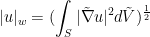
![\displaystyle |f|^2_v=max_{t\in [0,T]}\int_S|\tilde \nabla f|^2d\tilde V +\int_0^T\int_M |\frac{\partial f}{\partial t}|^2 d\tilde Vd t](https://s0.wp.com/latex.php?latex=%5Cdisplaystyle+%7Cf%7C%5E2_v%3Dmax_%7Bt%5Cin+%5B0%2CT%5D%7D%5Cint_S%7C%5Ctilde+%5Cnabla+f%7C%5E2d%5Ctilde+V+%2B%5Cint_0%5ET%5Cint_M+%7C%5Cfrac%7B%5Cpartial+f%7D%7B%5Cpartial+t%7D%7C%5E2+d%5Ctilde+Vd+t&bg=ffffff&fg=000000&s=0&c=20201002)
 ]
] ![{\nu^{k,\alpha,[0,T]}}](https://s0.wp.com/latex.php?latex=%7B%5Cnu%5E%7Bk%2C%5Calpha%2C%5B0%2CT%5D%7D%7D&bg=ffffff&fg=000000&s=0&c=20201002) is the set of
is the set of  in
in ![{\rho^{l,\alpha,[0,T]}}](https://s0.wp.com/latex.php?latex=%7B%5Crho%5E%7Bl%2C%5Calpha%2C%5B0%2CT%5D%7D%7D&bg=ffffff&fg=000000&s=0&c=20201002) with finite
with finite ![\displaystyle ||\cdot||_{\nu^{k,\alpha,[0,T]}}=||\cdot||_{\rho^{l,\alpha,[0,T]}}+|\cdot|_v](https://s0.wp.com/latex.php?latex=%5Cdisplaystyle+%7C%7C%5Ccdot%7C%7C_%7B%5Cnu%5E%7Bk%2C%5Calpha%2C%5B0%2CT%5D%7D%7D%3D%7C%7C%5Ccdot%7C%7C_%7B%5Crho%5E%7Bl%2C%5Calpha%2C%5B0%2CT%5D%7D%7D%2B%7C%5Ccdot%7C_v&bg=ffffff&fg=000000&s=0&c=20201002)


 , the limit exist and find a way to calculate it.
 .
. local-index thm
  .
. is a self-adjoint operator .
  .
.  .
. is symmetric
  is finite dimention
  is finite dimesion
  is finite dimension.
 :
:

 .
. over a compact manifold

 .
. -graded vector bundle
 ![{Str[D,K]=0}](https://s0.wp.com/latex.php?latex=%7BStr%5BD%2CK%5D%3D0%7D&bg=ffffff&fg=000000&s=0&c=20201002) .
.



 is independent with
  ,in fact:
![{\Longrightarrow \ D^2e^{-tD^2}=[D,D E^{-tD^2}]}](https://s0.wp.com/latex.php?latex=%7B%5CLongrightarrow+%5C+D%5E2e%5E%7B-tD%5E2%7D%3D%5BD%2CD+E%5E%7B-tD%5E2%7D%5D%7D&bg=ffffff&fg=000000&s=0&c=20201002) .
.![{[\ \ ,\ \ ]}](https://s0.wp.com/latex.php?latex=%7B%5B%5C+%5C+%2C%5C+%5C+%5D%7D&bg=ffffff&fg=000000&s=0&c=20201002) supercommunater
supercommunater ![{\Longrightarrow \ \frac{d}{dt}Str (e^{-tD^2})= -Str[D,D e^{-tD^2}]=0.}](https://s0.wp.com/latex.php?latex=%7B%5CLongrightarrow+%5C+%5Cfrac%7Bd%7D%7Bdt%7DStr+%28e%5E%7B-tD%5E2%7D%29%3D+-Str%5BD%2CD+e%5E%7B-tD%5E2%7D%5D%3D0.%7D&bg=ffffff&fg=000000&s=0&c=20201002)
 :
:
 for
for  .
.  . (detail in [BGV])


![{ D=\left[\begin{array}{ccc} 0 & D^- \\ D^+ & 0 \end{array}\right] \Longrightarrow D^2=\left[\begin{array}{ccc} D^-D^+ & 0\\ 0 & D^+D^- \end{array}\right] }](https://s0.wp.com/latex.php?latex=%7B+D%3D%5Cleft%5B%5Cbegin%7Barray%7D%7Bccc%7D+0+%26+D%5E-+%5C%5C+D%5E%2B+%26+0+%5Cend%7Barray%7D%5Cright%5D+%5CLongrightarrow+D%5E2%3D%5Cleft%5B%5Cbegin%7Barray%7D%7Bccc%7D+D%5E-D%5E%2B+%26+0%5C%5C+0+%26+D%5E%2BD%5E-+%5Cend%7Barray%7D%5Cright%5D+%7D&bg=ffffff&fg=000000&s=0&c=20201002) .
. is the heat trace invariants.
 ,and we want to proof:
 has a limit as
  index density.
 . We will write
  for the heat kernel associated to
  is a section of
  which is iso- morphic to
  . Using this isomorphism, we define a filtration on
  . Elements of
  are given 0-degree. Denote by
  the subbundle of
  .
. have degree less or equal to
  . In other words,
  . 2. If
  ,where
  denotes the
  restriction of the symbol map, then:

 of order less than n all vanish,in the other word:
 of dimension
 ![{CL_{n-1}(V) =[CL(V),CL(V)]}](https://s0.wp.com/latex.php?latex=%7BCL_%7Bn-1%7D%28V%29+%3D%5BCL%28V%29%2CCL%28V%29%5D%7D&bg=ffffff&fg=000000&s=0&c=20201002) .
. be a basis of
  . For any multi-index
  , denote by
  the Clifford product
  .Then the set
  is a basis for
  .If
.If ,there is at least one
  such that
  , and we have
![\displaystyle c(e_I)=-\frac{1}{2}[c_j,c_j c_I].](https://s0.wp.com/latex.php?latex=%5Cdisplaystyle+c%28e_I%29%3D-%5Cfrac%7B1%7D%7B2%7D%5Bc_j%2Cc_j+c_I%5D.+&bg=ffffff&fg=000000&s=0&c=20201002)
 as a characteristic form on
  where
where  denotes the symbol map and
  is the projection of
  onto the coefficient of
  if
if 
![{CL_{n-1}(V)=[CL(V),CL(V)]}](https://s0.wp.com/latex.php?latex=%7BCL_%7Bn-1%7D%28V%29%3D%5BCL%28V%29%2CCL%28V%29%5D%7D&bg=ffffff&fg=000000&s=0&c=20201002) and it never be empty because there is a natural defined supertrace on
and it never be empty because there is a natural defined supertrace on  .so the only thing we need to do is to determine the constant,in face we only need to calculate the supertarce on any non-zero element .for instance the chirality operator
  . We have that
  and therefore
  for all
  .
. section
  :
:

 . Let
. Let  exists and is obtained by taking the

 around a point
  . Near the diagonal, we use parallel transport to pull back the heat kernel
  which is a section of the vector bundle
  and define a new kernel
  , a section of
  for some twisting space
  . Using the symbol isomorphism
  , we can look at
  as a section of
  .
. .
. of theorem 1 which leads to a reformulation of Theorem 1.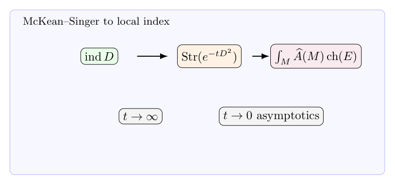
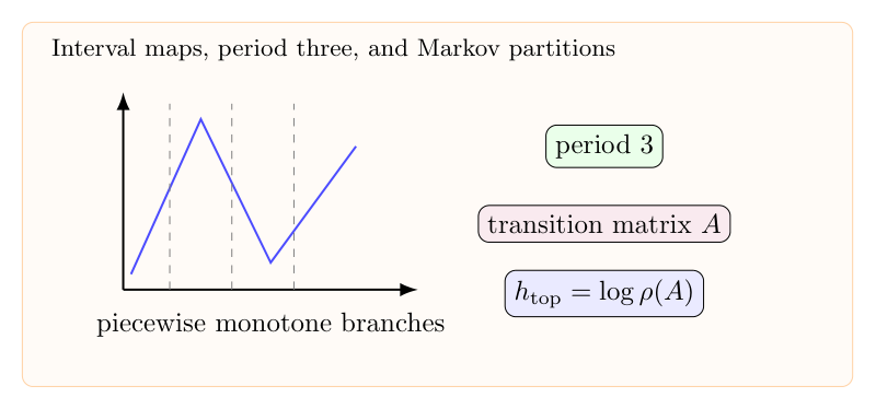
 have a period 3 point
  ,then
,then  ,there is a period n point for
  .
. case:
case: defined as the number of monotone interval of the map
  .
. .
. matrix
  .
.
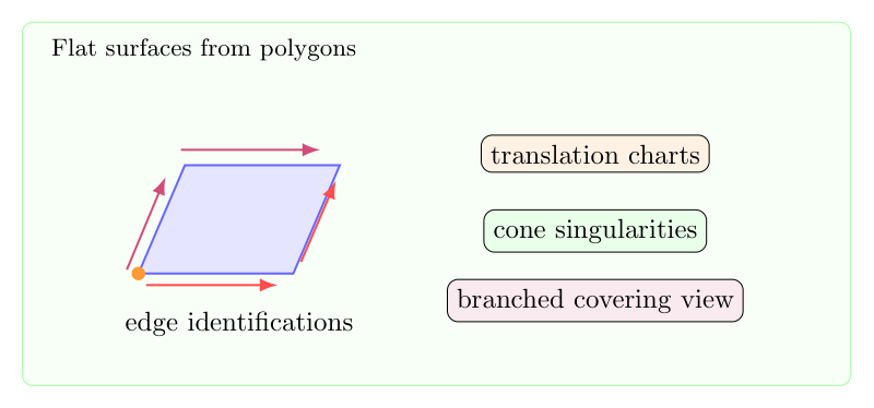
 with a (ramified in nontrivial case) map
 .
. is not ramified on
  is not ramified and defined a covering map.
 of M.and
 :
:
 campact,complete,Riemann manifold without boundary,dim
  .
.  is the Levi-civita connection on
  ,
, .
. genus form:
 is closed.
 is exact.
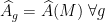 is a metric on M.
 is a dirac bundle.
 is dirac operator.
 the twisting curvature of
  . induce map:

![\displaystyle ch^{E / S}(E) = Str^{E /S}[exp(\frac{i}{2\pi}F^{E/S})] \in \Omega(M).](https://s0.wp.com/latex.php?latex=%5Cdisplaystyle+ch%5E%7BE+%2F+S%7D%28E%29+%3D+Str%5E%7BE+%2FS%7D%5Bexp%28%5Cfrac%7Bi%7D%7B2%5Cpi%7DF%5E%7BE%2FS%7D%29%5D+%5Cin+%5COmega%28M%29.&bg=ffffff&fg=000000&s=0&c=20201002)
 closed form.
 only depend on the topology of E.



 .
. with the norm
  is the sobolev space
  .
. in
in  is called
  ,assume
  is
is  ,
, called
  ,
, complete with the norm
  , of course
  .
. .
. ,satisfied
  ,where * is the Hodge-star operator ,
 is the
  1-form, iff one of
  is compact supp.
 .
. , When M is with smooth boundary,then
  ,assume M is complete (
 ,Gaffney proved(Ann. of Math , 60 ,1954,140-145),
 is self-adjoint operator,so
  make up a bounded self-adjoint operator semi group,by the self-adjoint operator theory,if
  is the spectrum measure of
 ,
, .when
.when  ,
,
 is basic on Weyl theory.
 : assume
  ,and
,and  ,
, ,satisfied:
 .to proof this,we first proof,in weak sense:
![{ \frac{\partial}{\partial t} (e^{-\Delta t} f) \\=\lim\limits_{\epsilon \rightarrow 0} \frac{1}{\epsilon} [\int \limits_0^\infty e^{-\lambda(t+\epsilon)}dE_{\lambda}(f)-\int\limits_0^\infty e^{-\lambda t} dE_{\lambda}(f)] \\=\lim\limits_{\epsilon \rightarrow 0}[\int\limits_0^A \frac{e^{-\lambda \epsilon}-1}{\epsilon} e^{-\lambda t} dE_{\lambda}(f)+\int\limits_A^\infty \frac{e^{-\lambda\epsilon}-1}{\lambda\epsilon} \lambda e^{-\lambda t}dE_{\lambda}(f)] \\=\int\limits_0^A -\lambda e^{-\lambda t} dE_{\lambda}(f) + O(Ae^{-At} \|f\|) \\ \longrightarrow \int\limits_0^\infty -\lambda e^{-\lambda t} dE_{\lambda}(f) \ as\ {A \ \rightarrow +\infty} \dotfill (\star).}](https://s0.wp.com/latex.php?latex=%7B+%5Cfrac%7B%5Cpartial%7D%7B%5Cpartial+t%7D+%28e%5E%7B-%5CDelta+t%7D+f%29+%5C%5C%3D%5Clim%5Climits_%7B%5Cepsilon+%5Crightarrow+0%7D+%5Cfrac%7B1%7D%7B%5Cepsilon%7D+%5B%5Cint+%5Climits_0%5E%5Cinfty+e%5E%7B-%5Clambda%28t%2B%5Cepsilon%29%7DdE_%7B%5Clambda%7D%28f%29-%5Cint%5Climits_0%5E%5Cinfty+e%5E%7B-%5Clambda+t%7D+dE_%7B%5Clambda%7D%28f%29%5D+%5C%5C%3D%5Clim%5Climits_%7B%5Cepsilon+%5Crightarrow+0%7D%5B%5Cint%5Climits_0%5EA+%5Cfrac%7Be%5E%7B-%5Clambda+%5Cepsilon%7D-1%7D%7B%5Cepsilon%7D+e%5E%7B-%5Clambda+t%7D+dE_%7B%5Clambda%7D%28f%29%2B%5Cint%5Climits_A%5E%5Cinfty+%5Cfrac%7Be%5E%7B-%5Clambda%5Cepsilon%7D-1%7D%7B%5Clambda%5Cepsilon%7D+%5Clambda+e%5E%7B-%5Clambda+t%7DdE_%7B%5Clambda%7D%28f%29%5D+%5C%5C%3D%5Cint%5Climits_0%5EA+-%5Clambda+e%5E%7B-%5Clambda+t%7D+dE_%7B%5Clambda%7D%28f%29+%2B+O%28Ae%5E%7B-At%7D+%5C%7Cf%5C%7C%29+%5C%5C+%5Clongrightarrow+%5Cint%5Climits_0%5E%5Cinfty+-%5Clambda+e%5E%7B-%5Clambda+t%7D+dE_%7B%5Clambda%7D%28f%29+%5C+as%5C+%7BA+%5C+%5Crightarrow+%2B%5Cinfty%7D+%5Cdotfill+%28%5Cstar%29.%7D&bg=ffffff&fg=000000&s=0&c=20201002)
 space,every step in the caculate make sence because of the dominating convergence theorem.
 exist. and our strategy is to proof any order of weak derivatives of it exist and then use the embedding theorem to prove it is smooth.
 (in weak sence),we need only to proof:
 we have:
 ,this is obvious,and similar we can proof that (in the weak sence):
 .
. is the laplace operator on
  .and we have proved
  ,and we know that
  .so we proved
 ,then:

 ,so derivatives is in classical sense.
 .
. ,and
,and  sufficed small.
 and its quasi fundamental solution (paramatrix)
  see next section for the serious definition
  ,
,
 ,and when
  suffice small,
 ,we have expansion:
 Riemann distance.
 ,for
,for  ,
,![{ e^{-\Delta\epsilon}P(x,y,t-\epsilon)-e^{-\Delta(t-\epsilon)}P(x,y,\epsilon)\\ = \int\limits_{\epsilon}^{t-\epsilon} \frac{d}{ds}(e^{-\Delta(t-s)} P(x,y,s))ds\\ =\int\limits_{\epsilon}^{t-\epsilon} [ \Delta e^{ -\Delta(t-s)P(x,y,s)} + e^{-\Delta(t-s)} \frac{\partial P}{\partial s}(x,y,s)]ds\\ =\int\limits_{\epsilon}^{t-\epsilon} e^{-\Delta(t-s)} \circ _xP(x,y,s)ds.}](https://s0.wp.com/latex.php?latex=%7B+e%5E%7B-%5CDelta%5Cepsilon%7DP%28x%2Cy%2Ct-%5Cepsilon%29-e%5E%7B-%5CDelta%28t-%5Cepsilon%29%7DP%28x%2Cy%2C%5Cepsilon%29%5C%5C+%3D+%5Cint%5Climits_%7B%5Cepsilon%7D%5E%7Bt-%5Cepsilon%7D+%5Cfrac%7Bd%7D%7Bds%7D%28e%5E%7B-%5CDelta%28t-s%29%7D+P%28x%2Cy%2Cs%29%29ds%5C%5C+%3D%5Cint%5Climits_%7B%5Cepsilon%7D%5E%7Bt-%5Cepsilon%7D+%5B+%5CDelta+e%5E%7B+-%5CDelta%28t-s%29P%28x%2Cy%2Cs%29%7D+%2B+e%5E%7B-%5CDelta%28t-s%29%7D+%5Cfrac%7B%5Cpartial+P%7D%7B%5Cpartial+s%7D%28x%2Cy%2Cs%29%5Dds%5C%5C+%3D%5Cint%5Climits_%7B%5Cepsilon%7D%5E%7Bt-%5Cepsilon%7D+e%5E%7B-%5CDelta%28t-s%29%7D+%5Ccirc+_xP%28x%2Cy%2Cs%29ds.%7D&bg=ffffff&fg=000000&s=0&c=20201002)
 ,and assume
  ,
,
 ,then
,then
 ,when
,when  ,so
,so  ,so
,so 
 and
and  have the same expansion .because
 so
so  ,we have:
 is fix and
  , so
, so
 is from the operator
  .
.
 so
so .
. and
and 
 is
is  .
.
 .(the length of geodesic connect
  ).
). only depend on






![\displaystyle (\Delta -\frac{\partial}{\partial t})u_N = \frac{\psi}{t}\sum\limits_{k = 0 ... N} [ \Delta \phi_{k-1} -(k+\frac{r}{2}\frac{d \ log\sqrt{g}}{dr})\phi_k -r\frac{d \phi_k}{dr}]t^k ,](https://s0.wp.com/latex.php?latex=%5Cdisplaystyle+%28%5CDelta+-%5Cfrac%7B%5Cpartial%7D%7B%5Cpartial+t%7D%29u_N+%3D+%5Cfrac%7B%5Cpsi%7D%7Bt%7D%5Csum%5Climits_%7Bk+%3D+0+...+N%7D+%5B+%5CDelta+%5Cphi_%7Bk-1%7D+-%28k%2B%5Cfrac%7Br%7D%7B2%7D%5Cfrac%7Bd+%5C+log%5Csqrt%7Bg%7D%7D%7Bdr%7D%29%5Cphi_k+-r%5Cfrac%7Bd+%5Cphi_k%7D%7Bdr%7D%5Dt%5Ek+%2C&bg=ffffff&fg=000000&s=0&c=20201002)




 . and:
 ,
, :
:



 is the quasi fundamental solution of heat equation. from the equation:

 has suffise high zero ,then so is the solution of heat equation,so
  can approximate heat equation to any order.
 :
:
 ,use the stokes formula and maximal value principle to proof
  : assume
  ,and
,and . proof is similar to
  (heat kernel comparision theorem,Cheeger-Yau).:
 ,
, , heat kernel of
  and heat kernel
  of geodesic ball
  in space form satisfied:
 .and the two lemma.
  : assume
  is a orthonormal basis of special function on
  is the corresponding spectrum,then the fundamental solution (heat kernel) has the expansion:
 ,
,
 be a compact
  Riemannian manifold of dimension
  , let
, let  be an
be an  latex N \phi_{\lambda} =\{x:\phi_{\lambda}(x)=0\}$
 denote its
  -dimensional Riemannian hypersurface measure. In this note we prove:
 ,there exists a constant
  so that:

 ,
,

 ,use divergence theorem:
 in theorem 2,we have:
 ,$||\nabla\phi_{\lambda}||_{\infty}$ ,this two guys are easy to get good estumate….and we will get a lower bound estimate of measure of nodal set:

 norm of

 上的加倍映射,旋转映射以及
 上的平移映射。
 的singular point,也就是
 的地方附近的环绕数计算,还有一些scalling变换或者是一些多尺度的问题里。\\
 open,
open, 或者
或者 开集,
开集, ,
, \\
\\ 是一个
是一个 集合
集合 这个集合是$T$不变的,第二点是注意到transitive point可以通过选取一组开集集进行描述从而有集合等式:
 所有的点都是transitivity point。\\
 不变的集合满足zorn lemma,所以有最小元\\
 分成若干个类,一定存在一个类存在任意长等差数列。\\
 装备上平移这个同胚构成的动力系统就够了,等差数列的存在性等价于若干个可以交换的映射,其实就是平移的步长不一样下的都回到原始值附近,这是birkhoff回复定理能够告诉我们的。\\
 在底空间上作用是transitive的,
 在第一层纤维上的作用是transitive的,依次类推。由于交换性可以导致在每一个section上
 ,$T^iT^j=T^jT^i$,并不存在满足某种”一致”minimal的子空间。但是我们知道多重回复定理是对的。\\
 ,最后证明动力系统之间的半共轭会导致熵之间的不等式。
 情况的技巧
情况的技巧 这个会化简为简单的情况,再加上凸性。
 Boudary正则性的区域上特征函数的的谱我们有没有好的刻画,这其中能不能蕴含这个区域的几何信息。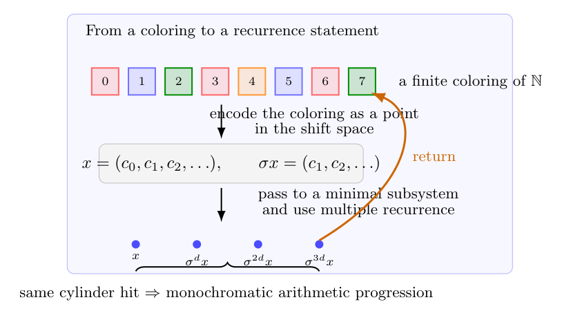

 Bourgain-Sarnak-Ziegler定理可以视为Vingrodov均值定理的有限版本。