博客

  • Gromov-Hausdorff 距离笔记:不同维球面之间能多近?

    旧博客原文

    原题:How to compute the Gromov-Hausdorff distance between spheres $latex S_n$ and $latex S_m$?

    There is the question, because when we consider the Gromov-Hausdorff distance, we must fix the metric, so we use the natural metric induced from the embedding \mathbb{S}_n \to \mathbb{R}^{n+1}. Is it possible for us to compute the Gromov-Hausdorff distance d_{G-H}(\mathbb{S}_n,\mathbb{S}_m) for two different spheres \mathbb{S}_n and \mathbb{S}_m, m\neq n?

    For example if we want to calculate d_{G-H}(\mathbb{S}_2,\mathbb{S}_3)=\inf_{M,f,g}d_{M}(\mathbb{S}_2,\mathbb{S}_3), where M ranges over all possible metric space and f:\mathbb{S}_2\to M and g:\mathbb{S}_3\to M range over all possible isometric (distance-preserving) embeddings.

    At least we can embed \mathbb{S}_2,\mathbb{S}_3 into \mathbb{R}^3 in a canonical way. This will lead to a upper bound: d_{G-H}(\mathbb{S}_2,\mathbb{S}_3)\leq \sqrt{2}. And in general case we have d_{G-H}(\mathbb{S}_m,\mathbb{S}_n)\leq d_{G-H}(point,S_m)+d_{G-H}(point,S_n)\leq 2,\forall 0\leq n\leq m. But it is difficult to get a lower bound control for me. Because we need to take the inf in all possible metric spaces M. Especially I conjecture d_{G-H}(\mathbb{S}_m,\mathbb{S}_n)\geq \lambda_{m,n}\frac{m-n}{m},\forall 0\leq n\leq m, where \liminf_{m,n\to \infty}\lambda_{m,n}>0.

    I only know the knowledge of Gromov-Hausdorff from Peterson’s Riemann Geometry. Unfortunately there is not enough information to compute the Gromov-Hausdorff distance, so this problem may be very stupid, I will appreciate any pointer.


    And we know for the case S_n,S_m, if n,m is very near to each other,then the two space should be more near, and there is a canonical embed S_0\subset S_1 \subset S_2 ....\subset S_n \subset .... So it is natural to conjecture if m,n is very near then the distance d_{G-H}(S_n,S_m) is very small. I have a very rough strategy to prove the conjecture, that is inspired by the Nash embedding theorem. I just mean if we consider the problem in this frame d_{G-H}(S_n,S_m)=\inf_{M,g,f}(d_M(f(S_n),g(S_m))) then the difficult is the deformation space of M,g,f is too large. so the first step is to establish a regular lemma, to prove the function d_M(f(S_n),g(S_m)) is continues under the small perbutation of M and reduced to the situation of space $M,g,f$ with very nice regularity. the second part is to embed M to a big euclid space R^N as subspace, and the embedding stay the length of geodesic.locally this is determine by a group of pde:u_i(x)u_j(x)=g_{ij}(x),at least in the cut locus.but there should be some critical point,and I do not know how to deal with them.the third,i.e. the last step is to calculate d_{G-H}(S_n,S_m) in the very some deformation space M,f,g.

    @Mark Sapir,Appreciate for help!I am reading the article you point out,it seems this article mainly focus on investigating the Gromov-Hausdorff limit space of a sequence of hyperbolic group equipped with modified G-H metric defined in 2.A with some special condition to ensure the limit space exists.and take a sequences corvarage to the limit space,the hyperbolic property and some other thing is stayed by the process of take limit.
    @Mark Sapir,So it is natural for us to investigate the original space by some information from the limit space.there is a series of bi-product state in 3.B.but I do not see where the author exactly calculate some groom-hausdorff distance of two different space,may you point out it?appreciate again!
    @MarianoSuárez-Álvarez,Corrected, thanks.

    Y:
    I fixed numerous typos. In particular, you should use spacing after each punctuation mark; capitals to begin sentences and names.

    H:
    Thank you very much for helping me to correct the mistakes! I will know how to write in a correct style.

    Y:
    23.1k
    Your conjecture would imply that the GH distance is unbounded. But it’s clearly bounded, since the GH distance of any sphere to a point is equal to 2 (when the sphere is endowed with the restriction of Euclidean distance, as you seem to assume, or \pi when endowed with geodesic distance) and hence the GH distance between any two spheres is \le 4.

    H:
    73
    You are right,In fact if we use the canonical embed, then we can get d_{G-H}(S_n,S_m)\leq 2 by another equivalent definition of GH distance.I confuse the geometry picture of the pairs T_n,S_n with the pairs S_n,S_m,for S_n,S_m case,I thick the seems correct conjecture will be d_{G-H}(S_n,S_m)\sim \frac{m-n}{m},0\leq n\leq m,m,n\to \infty.

    Y:
    16:37
    Clearly from standard embeddings we get d_{GH}(S_n,S_m)\le\sqrt{2} for all n,m\ge 0. Would it be reasonable to simply conjecture that it’s an equality whenever n\neq m?

    H:
    73
    Yeah, you are right,d_{G-H}(S_n,S_m)\leq \sqrt{2} for all n,m\geq 0.I find the interesting problem when I want to find a toy model of a kind of problem,roughly speaking is to investigate a map f:X\to Y from low-dimensions space X to high-dimension space Y stay some affine structure of the low-dimension space X. This structure could have some control by the distance function on the low-dimension space, so if we can get some control on the variation of the Energy of distance function, this will share some line on the original problem I consider.
    And we know for the case S_n,S_m, if n,m is very near to each other,then the two space should be more near, and there is a canonical embed S_0\subset S_1 \subset S_2 ....\subset S_n \subset .... So it is natural to conjecture if m,n is very near then the distance d_{G-H}(S_n,S_m) is very small. .
    I have a very rough strategy to prove the conjecture, that is inspired by the Nash embedding theorem. I just mean if we consider the problem in this frame d_{G-H}(S_n,S_m)=\inf_{M,g,f}(d_M(f(S_n),g(S_m))) then the difficult is the deformation space of M,g,f is too large. so the first step is to establish a regular lemma, to prove the function d_M(f(S_n),g(S_m)) is continues under the small perbutation of M and reduced to the situation of space M,g,f with very nice regularity.
    The second part is to embed M to a big euclid space R^N as subspace, and the embedding stay the length of geodesic.locally this is determine by a group of pde:u_i(x)u_j(x)=g_{ij}(x),at least in the cut locus.but there should be some critical point,and I do not know how to deal with them.the third,i.e. the last step is to calculate d_{G-H}(S_n,S_m) in the very some deformation space M,f,g.
    I need come back to explain why we expect the groom-hausdorff distance d_{G-H}(S_d,S_m),0\leq n\leq m should be much small than \sqrt 2 when frac{n}{m} is small.

    Let consider a toy model of the problem,in a graph model,i.e. now we do not consider to take the Infimum in all space but in discrete space endow with metric. this can be view as a complete graph equipped metric, i.e. M=\{(G,d_G)\}. So there is also some space very like S_n,$S_m$ in the Euclid space, Let remark them as G_{S_n},G_{S_m}.
    , oberseve that (G,d_G)\in M then (G,\hat d_{G})\in M,\hat d_{G} is a scaling of d_Gso it is natural to consider a cut off of M,called M_{\lambda} which is just a subset of M and satisfied if (G,d_G)\in M_{\lambda},then \inf_{x\neq y}d_{G}(x,y)\geq d.
    Now,in the space M_{\lambda} let us consider a Distance distribution:\mu_G((a,b))=\frac{\#\{x,y\in G|a<d_G(x,y)<b\}}{\#G\times G}. Then this distribution will give us some information of the distance of the two different set G_1,G_2 in M_{\lambda}.
    (removed)
    Now,in the space M_{\lambda} let us consider a Distance distribution:\mu_G((a,b))=\frac{\#\{x,y\in G|a<d_G(x,y)<b\}}{\#G\times G}. Then this distribution will give us some information of the distance of the two different set G_1,G_2 in M_{\lambda}.
    and obviously we will see that if n,m is close,then the distribution of fuzzy approximation G_{S_n},G_{S_m} is near, and the reverse is also true. I think this can explain why the conjecture d_{G-H}(S_n,S_m) =O(\frac{m-n}{m}) may be right.


    by the way,it is a very good exercise to proof d_{G-H}(S_n,S_0)=1,\forall n\in N^*.



    补充说明

    以下是新整理的中文说明;上方旧博客原文保持不变。

    问 $S^n$ 和 $S^m$ 的 Gromov-Hausdorff 距离,第一步必须先固定 metric。球面可以带内蕴测地距离,也可以带作为欧氏空间子集的 chordal distance;不同选择会给出不同数值。真正稳定的对象不是某个嵌入,而是所有可能 correspondences 的 distortion。
    Gromov-Hausdorff 距离笔记:不同维球面之间能多近?
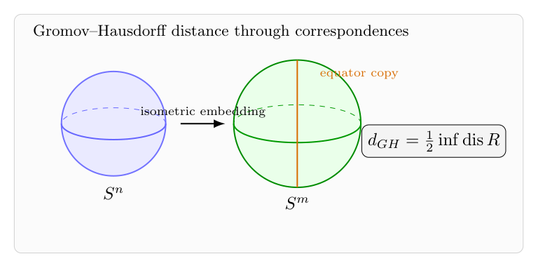
    比较不同维球面时,标准嵌入只给出上界;真正的 GH 距离要在所有 correspondences 上取最优。

    1. 定义提醒

    紧 metric spaces $X,Y$ 的 Gromov-Hausdorff 距离可以用 correspondences 表示:

    $$d_{GH}(X,Y)=\frac12\inf_R \operatorname{dis}(R),$$

    其中 $R\subset X\times Y$ 是 correspondence,distortion 定义为

    $$\operatorname{dis}(R)=\sup_{(x,y),(x’,y’)\in R}
    \bigl|d_X(x,x’)-d_Y(y,y’)\bigr|.$$

    这一定义强调:我们不是只比较两个空间在某个欧氏空间中的位置,而是允许把它们同时嵌入任意 metric space,再取最优比较。

    2. 先用标准嵌入给上界

    若 $n

    $$d_{GH}(S^n,S^m)\le \sqrt2.$$

    若用 geodesic metric,对应上界是 $\pi/2$。这只是上界,不自动说明最优。

    3. 为什么不能猜它随维数增长

    一个容易犯的错误是认为维数差越大,距离越大。但 GH 距离由直径控制。对任意紧空间 $X$,

    $$d_{GH}(X,\{\ast\})=\frac12\operatorname{diam}(X).$$

    因此两单位球面之间的 GH 距离总是被一个统一常数控制,不可能随着 $m-n$ 无界增长。维数差体现为拓扑和覆盖数的差异,但 GH 距离本身仍然是 metric 层面的量。

    4. 下界为什么难

    要证明 equator 嵌入给出的上界是最优,需要排除所有更聪明的 correspondences。这通常要找一个 metric invariant,例如 covering number、packing number、waist phenomenon 或同调信息,说明低维球面无法在小 distortion 下模拟高维球面。

    例如,如果 $S^m$ 中有许多两两相距较远的点,而 $S^n$ 在同样尺度下容纳不了这么多点,就可以得到下界。这类 argument 本质上是把维数信息转化成 packing 数据。

    5. 一个合理的 toy problem

    这个问题真正有意思的地方在于,它是“低维空间如何嵌入高维空间并保留距离结构”的 toy model。若把球面换成带变形 metric 的流形,还会涉及 Nash embedding、cut locus、距离函数能量的变化以及正则性问题。

    所以比较 $S^n$ 和 $S^m$ 不只是为了得到一个数值;它逼迫我们区分三件事:具体嵌入给出的 Hausdorff 上界、抽象 GH 距离的最优 correspondence、以及维数信息如何通过 metric invariant 被读出来。

  • k-curvature 方程的正则性:连续性方法、屏障函数与边界估计

    旧博客原文

    原题:Regularity of k-curvature equation

    this is a note after reading the article”” of Cafferalli.

    in his article,a large type of fully nonlinear elliptic equation has been established.in particular,including the k-curvature equation.and use the continue method,we just need to establish a ingredient estimate,C^2 estimate in the interior and C^2 estimate near the boundary.we establish these estimate step by step,base on construct special flexible function and use the maximum principle to establish the first and second estimate,for the C^2 estimate near the boundary we need to investigate the influence of permutation on the boundary carefully.


    补充说明

    以下是新整理的中文说明;上方旧博客原文保持不变。

    $k$-curvature 方程属于完全非线性椭圆方程。典型形式可以写成

    $$F(D^2u,Du,u,x)=\sigma_k(\kappa[u])=\psi(x),$$

    其中 $\sigma_k$ 是主曲率的第 $k$ 个初等对称函数。Caffarelli-Nirenberg-Spruck 一类理论的核心是:在合适凸性锥中建立先验估计,然后用连续性方法得到解。

    k-curvature 方程的正则性:连续性方法、屏障函数与边界估计
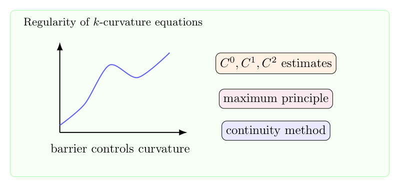
    k-curvature 方程的正则性证明依靠连续性方法、屏障函数、最大值原理和边界二阶估计。

    1. 连续性方法

    把目标方程嵌入一族方程 $F_t(u)=0$。若 $t=0$ 可解,开性来自线性化算子的可逆性,闭性则依赖统一先验估计。于是关键变成:

    $$\|u\|_{C^{2,\alpha}}\le C.$$

    2. 内部估计

    $C^0$ 和 $C^1$ 估计通常来自最大值原理与几何屏障。二阶估计更微妙,需要对最大特征值构造辅助函数,并利用方程的凹性抵消坏项。

    3. 边界估计

    边界附近最难的是混合二阶导数和法向二阶导数。这里要仔细利用边界曲率、可容许锥条件,以及对称函数 $\sigma_k$ 在坐标置换下的结构。

    4. 正则性升级

    一旦得到一致椭圆性和 $C^2$ 控制,可以通过 Evans-Krylov 定理得到 $C^{2,\alpha}$,再用 Schauder theory 提升到更高正则性。整个证明的脊梁是:屏障函数给低阶控制,最大值原理给二阶控制,椭圆正则性完成升级。

  • Wolff 的 Kakeya maximal estimate:X-ray 估计与三维障碍

    旧博客原文

    原题:Kakeya conjecture (Tomas Wolff 1995)

    There is a main obstacle to improve the kakeya conjecture,remain in dimension 3,and the  result established by Tomas Wolff in 1995 is almost the best result in R^3 even until now.the result establish by Katz and Tao can be view as a corollary of Wolff’s X-ray estimate.

    For f\in L_{loc}^1(R^d),for 0<\delta<1:

    f_{\delta}^*:P^{d-1}\longrightarrow R.f_{\delta}^*(e)=\sup_{T}\frac{1}{|T|}\int_{T}|f|.

    T is varise in all cylinders with length 1.radius \delta.axis in the e direction.

    f_{\delta}^{**}:R^d\longrightarrow R.f^{**}_{\delta}(x)=sup_{T}\frac{1}{|T|}\int_{T}|f|.

    T varise in cylinders contains x,length 1,radius \delta.

    Keeping this two maximal function in mind,we give the statement of the Kakeya maximal function conjecture:

    ||M_{\delta}f||_d\leq C_{\epsilon} \delta^{-\epsilon}||f||_d

    Where M_{\delta}=f_{\delta}^* or M_{\delta}=f_{\delta}^{**}.

    Because we have the obviously 1-\infty estimate:

    ||f^*_{\delta}||_{\infty}\leq\frac{||f||_1}{|T|}=\delta^{1-d}||f||_1.

    ||f^{**}_{\delta}||_{\infty}\leq\frac{||f||_1}{|T|}=\delta^{1-d}||f||_1.

    So by the Riesz-Thorin interpolation we have:

    ||M_{\delta}f||_{q}\leq C_{\epsilon}\delta^{-(\frac{d}{p}-1+\epsilon)}||f||_p.           (*)

    for 1\leq p\leq d,q\leq(d-1)p'.the task is establish (*) for (p,q) as large as posible in the range.

    for the 2 dimension case,the result is well know.the key estimate is:

    \sum_{j}|T_i\cap T_j|\leq log(\frac{1}{\delta})|T_i|

    for d\geq 3 case,the main result of Wolff is:

    ||M_{\delta}f||_q\leq C_{\epsilon}\delta^{-(\frac{d}{p}-1+\epsilon)}||f||_p

    hold for p=\frac{d+2}{2}.q=(d-1)p'. M_{\delta}=f_{\delta}^* or f_{\delta}^{**}.

    Now we sketch the proof.

    prove f_{\delta}^*,f_{\delta}^{**} cases together.

    We can make some reduction:

    the first one is we can assume the sup of f is in a fix compact set.

    the second is instead of consider f_{\delta}^{**},we can consider f_{\delta}^{***}(x)=\sup_{T}\frac{1}{|T|}\int_T|f|.

    where T varies in all cylinder with radius \delta,length 1,axis \frac{\pi}{100} with a fix direction.

    the first reduction is obvious(why?)

    the second reduction rely on a observe:

    ||f_{\delta}^{***}||_q\leq A(\delta)||f||_p          \Longrightarrow    ||f_{\delta}^{**}||_q\leq CA(\delta)||f|_p

    this is just finite cover by rotation of the coordinate and triangle inequality.

    now we begin to establish a frame and put the two situations f_{\delta}^*,f_{\delta}^{***} into it.

    Let M(d,1) be all line in R^d.

    then M(d,1)=R^d\times S^{d-1}/\sim is a 2d-2 dim manifold.

    M(d,1)\longrightarrow P^{d-1}

    l \longrightarrow  e_l

    e_l is the line parallel to l.and the middle point is original.

    dist(l_1,l_2)\sim \theta(l_1,l_2)+d_{mis}(l_1,l_2).


    Wolf axiom:

    (A,d) metric space.

    \mu(D(\alpha,\delta)) \sim \delta^m.\alpha\in A.\delta \leq diam(A).

    for certain m\in R^+.

    \forall \alpha\in A.F_{\alpha} \subset M(d,1) is given.and \bar{\cup_{\alpha}F_{\alpha}} is compact.

    d(\alpha,\beta)\lesssim inf_{l\in F_{\alpha};m\in F_{\beta}}dist(l,m) for all \alpha,\beta \in A.

    If f:R^d\longrightarrow R then we define M_{\delta}f:A\longrightarrow R by

    M_{\delta}f(\alpha)=\sup_{l\in F(\alpha)}\frac{1}{|T_{l}^{\delta}|}\int_{|T^{\delta}_l|}|f|.

    Property (**):

    If l_0\in \cup_{\alpha F_{\alpha}}. \Pi is a 2-plane.containing l_0and if \sigma \geq \delta and if \{\alpha_j\}_{j=0}^N is a \delta-seperated subset of A and for each j,there is l_j\in F_{\alpha_j} with dist(l_j,M(\Pi,l))<\delta and dist(l,l_0)<\sigma.then

    N\leq \frac{C\sigma}{\delta}


    补充说明

    以下是新整理的中文说明;上方旧博客原文保持不变。

    Wolff 1995 年的 Kakeya maximal estimate 是三维 Kakeya 理论中的经典结果。它把 tubes 的重叠问题转化为 maximal function 和 X-ray transform 的估计。

    Wolff 的 Kakeya maximal estimate:X-ray 估计与三维障碍
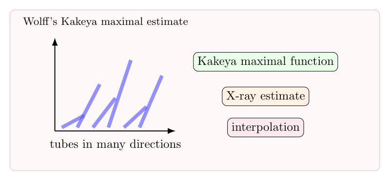
    Wolff 的 Kakeya maximal estimate 通过 X-ray 型平均和 incidence 几何控制 tubes 的重叠。

    1. Kakeya maximal function

    给定方向 $\omega$,考虑沿 $\omega$ 方向、半径 $\delta$、长度 $1$ 的 tube。Kakeya maximal function 粗略写为

    $$f_\delta^\ast(\omega)=\sup_{T\parallel\omega}\frac1{|T|}\int_T |f(x)|\,dx.$$

    猜想要求在尽可能大的 $p$ 范围内控制 $\|f_\delta^\ast\|_{L^q(S^{n-1})}$。

    2. 平凡估计与插值

    最直接的 $L^1$ 或 $L^\infty$ 估计通常太弱。通过 Riesz-Thorin interpolation 可以得到一些中间结果,但要接近 Kakeya 猜想,需要利用 tubes 的几何排列。

    3. X-ray transform

    X-ray transform 沿直线积分函数。Kakeya maximal function 可以看作对有限厚度 tubes 的 X-ray 型平均。Wolff 的估计用几何 incidence 控制这些平均的重叠。

    4. 归约步骤

    证明中可以把 tubes 限制在固定紧区域,并把方向分成有限个坐标 patch。这样 maximal function 可由有限方向族上的 tube averages 控制。

    5. 三维障碍

    三维最大的困难是 tubes 可以形成复杂 ruled surface 或 hairbrush 结构,普通 pairwise intersection 估计不够。Wolff 的结果抓住了这类结构的第一层几何约束,为 Katz-Tao 的后续改进提供了基础。

  • Julia set 的 Hausdorff 维数能否等于 2?

    旧博客原文

    原题:Julia set

    There is a major open problem:

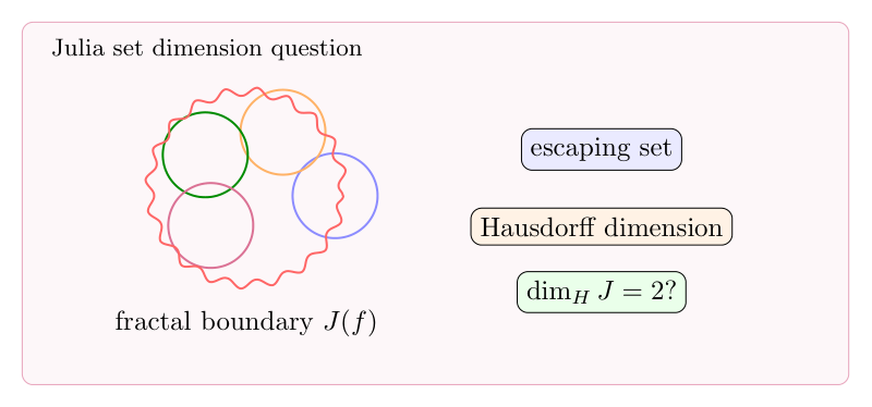
    Is there a polynomial f(z) such that the julia set T(J) of  mapT:z\longrightarrow f(z) satisfied the hausdorff dimension of J equal to 2?

    补充说明

    以下是新整理的中文说明;上方旧博客原文保持不变。

    复动力系统中的 Julia set 是迭代多项式

    $$f^{\circ n}(z)$$

    稳定性发生断裂的边界。一个自然问题是:是否存在多项式 $f$,使得 Julia set 的 Hausdorff 维数等于 $2$?也就是说,它虽然可能没有面积,却在维数意义上填满平面。

    Julia set 的 Hausdorff 维数能否等于 2?
    Julia set 的满 Hausdorff 维数问题连接复动力系统、分形几何和非一致双曲性。

    1. Fatou set 与 Julia set

    Fatou set 是迭代族正常的区域,Julia set 是它的补集。对 $f(z)=z^2+c$ 这样的二次多项式,Julia set 的形状会随参数 $c$ 发生剧烈变化。

    2. 维数为什么可能接近 2

    双曲多项式的 Julia set 往往有清晰的膨胀结构,维数可以通过压力函数计算。若系统接近抛物或临界退化,膨胀变弱,轨道在小尺度上停留更久,维数可能被推高。

    3. 等于 2 的含义

    $\dim_H J(f)=2$ 不等于说 $J(f)$ 有正面积。Hausdorff 维数为 $2$ 只说明它在任意小尺度上足够复杂;Lebesgue 面积是否为正是更强的问题。

    4. 研究路线

    一种思路是构造参数序列,使 Julia set 的维数趋近 $2$,再分析极限是否保持多项式动力系统的性质。另一种思路是研究临界轨道的回归速度和尺度几何,寻找能够制造满维数的非一致双曲机制。

  • 用互不相交闭区间覆盖半开区间:Ostrowski 表示与有效均匀分布

    旧博客原文

    原题:Covering a non-closed interval by disjoint closed intervals

    this note will talk about the Ostrowski representation and approximation by continue fraction.

    As well-known,by the Weyl criterion,\{n\alpha\} is uniformly distribution in [0,1] iff \alpha\in R-Q.

    i.e. we have:\forall 0\leq a\leq b\leq 1,we have:

    \lim_{N\to \infty}|\{1\leq n\leq N|\{n\alpha\}\in [a,b]\}|=(b-a)N+o(N).

    but this will not give the effective version.i.e. we do not the the more information about the decay of o(N).

    we will give a approach of effective version of \alpha with smooth condition by give another proof of the uniformly distribution (in fact to to decomposition the interval [a,b] in to a finite sums of special intervals).and get the result:

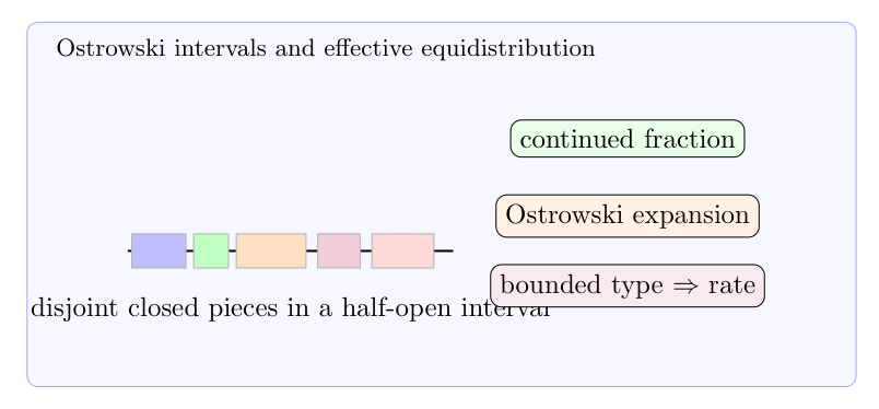
    D_N=\int_{M}D_N(\theta)d\mu=\int_Msup_{0<a<b<1}|\sum_{n=1}^{N}\chi_{(a,b)}(\{\theta n \})-N(b-a)|d\mu\sim O(log N)

    if the term in the continuous fraction of \alpha have a up bound.this is so called \alpha is smooth.


    补充说明

    以下是新整理的中文说明;上方旧博客原文保持不变。

    讨论无理旋转 $x\mapsto x+\alpha$ 的均匀分布时,Weyl criterion 告诉我们

    $$\frac1N\sum_{n\le N}e(k n\alpha)\to0,\qquad k\ne0.$$

    但这个判别法本身并不给出非常几何的有效误差。若想知道轨道落入某个区间 $I$ 的次数和 $N|I|$ 相差多少,就需要把区间和时间长度一起分解得更细。

    用互不相交闭区间覆盖半开区间:Ostrowski 表示与有效均匀分布
    Ostrowski 表示把轨道长度分解成连分数分母尺度,半开区间也可以拆成有限个互不相交的闭区间来控制端点误差。

    1. 半开区间为什么麻烦

    区间若不是闭的,端点会造成计数上的小麻烦;但在动力系统里,端点通常只贡献有限误差。因此可以把半开区间分解成有限个互不相交的闭区间,再把端点误差单独处理。

    2. 连分数与最佳逼近

    设 $\alpha=[a_0;a_1,a_2,\ldots]$,其收敛分母为 $q_j$。最佳逼近性质说明,长度约为 $\|q_j\alpha\|$ 的小区间正好对应旋转轨道的自然尺度。

    Ostrowski 表示把整数 $N$ 写成

    $$N=\sum_j b_j q_j,$$

    其中系数 $b_j$ 由连分数项控制。于是前 $N$ 次轨道可以分成若干个以 $q_j$ 为长度的块。

    3. 有效均匀分布

    若 $\alpha$ 的连分数项有一致上界,也就是 bounded type,那么每个尺度的坏误差都不会积累得太快。这样可以得到 Denjoy-Koksma 型估计:

    $$\left|\sum_{n

    这就是原来想要的“smooth”或有效版本:不仅知道趋于均匀,还知道偏差怎样增长。

  • Heat flow 与多项式零点:从变形思想到 Riemann Hypothesis 的 toy model

    旧博客原文

    原题:Heat flow and the zero of polynomial-a approach to Riemann Hypesis

    this is a note after reading the blog:Heat flow and the zero of polynomial.

    1.instead of consider the original version:

    \partial_{zz}f(z,t)=\partial_tf(z,t).

    consider the corresponding “equidistribution version” is also interesting:

    \partial_{zz}f(z,t)=\theta(z,t)\partial_tf(z,t),especially \theta(z,t)=e^{2\pi i\alpha t},\alpha\in R-Q.

    2.

    where f(z)=z^n+a_{n-1}z^{n-1}+...+a_1z+a_0.

    f(z,t)=\sum_{k=1}^n\sum_{0\leq m\leq k-2,2|k-m}\frac{k!}{m!(k-m)!}z^mt^{k-m}.

    =\sum_{k=1}^m\sum_{0\leq m\leq k-2,2|k-m}C_k^mt^{k-m})z^mt^{k-m}

    \sum_{m=0}^{n-2}(\sum_{k=m,2|k-m}^nC_k^mt^{k-m})z^m.

    rescaling:

    F_t:(z_1(t),...,z_n(t))\longrightarrow (\frac{z_1(t)}{t},...,\frac{z_n(t)}{t}).

    F_t\cdot f(z,t)=\sum_{m=0}^{n-2}(\sum_{k=m,2|k-m}^nC_{k}^mt^{k-n})z^m.

    \lim_{t\to \infty}F_t\cdot f(z,t)=\sum_{m=0,2|n-m}^{n-2}C_n^mz^m.(*)

    even term \longrightarrow constant.(after renormelization)

    odd term \longrightarrow 0(invariant).so at least the sum zeros of is invarient.

    by the algebraic fundamental theorem,we have n zero \{z_1,...,z_n\}of (*).

    until now,we already now if the n zeros is distinct,then because the energy is the energy is the same and the entropy is increase so \exists T>>0,\forall t_i,t_j>T,\{t>T|z_i(t)\} \cap \{t>T|z_j(t)\}=\emptyset.\lim_{t\to \infty}|z_i(t)|=\infty and \lim_{t\to \infty}arg(z_i(t))=z_i.

    but how to know the information of the change of direction at “blow up” time?

    1.change direction only at blow up.

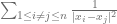
    2.energy invariant \sum_{1\leq i\neq j\leq n}\frac{1}{|x_i-x_j|^2}.

    3.general philosophy

    deformation some function under some evolution equation, such like heat equation,wave equation,shrodinger equation.and there is some conversion thing under the equation,and some quantity that could calculate directly such like the trace of spectral.

    4.difficultis

    this philosophy could generate to the analytic function case,but to make the limit case(I only know how ti deal with this now)coverage.we need very good control on the coefficient.

    and to investigate the change of direction at blow up point maybe we need some knowledge about the burid group.


    补充说明

    以下是新整理的中文说明;上方旧博客原文保持不变。

    用 heat flow 研究多项式零点,是理解更复杂解析函数零点问题的一个 toy model。基本思想是:让函数随时间演化,观察零点如何移动,以及哪些量在演化中保持或单调。

    Heat flow 与多项式零点:从变形思想到 Riemann Hypothesis 的 toy model
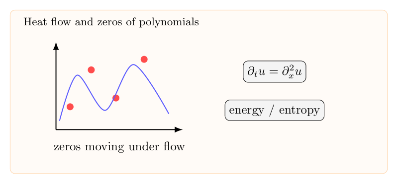
    heat flow 让多项式零点随时间运动,提供研究零点实性和不变量的 toy model。

    1. 多项式的 heat deformation

    设 $P(x)$ 是多项式,考虑

    $$\partial_t u=\partial_x^2u,\qquad u(0,x)=P(x).$$

    因为 heat operator 保持多项式空间,$u(t,x)$ 仍然是多项式。其零点随 $t$ 移动。

    2. 不变量与单调量

    某些系数组合在演化中保持不变,另一些量具有单调性。例如最高次项不变,低阶偶次项会随 heat flow 改变。零点的质心或某些对称量可能保持。

    3. 零点碰撞

    若零点始终实且互异,运动图像较清楚;真正困难发生在零点碰撞或分裂时。此时需要理解 blow-up 时间附近的方向变化。

    4. 与 Riemann Hypothesis 的类比

    de Bruijn-Newman 常数研究的是 Xi 函数在 heat flow 型变形下零点保持实的临界时间。多项式模型不能证明 RH,但能展示同一种哲学:通过演化方程追踪零点几何。

    5. 需要的估计

    要从多项式推广到整函数,必须控制系数、增长阶和极限过程。多项式情形的代数基本定理给出有限零点;整函数情形需要更强的紧性和零点分布估计。

  • 三维 Kakeya 猜想:hairbrush、密度递降与 Katz-Tao 思路

    旧博客原文

    原题:Kakeya conjecture in R^3

    Kakeya conjecture in R^3 is very subtle.in fact wolff stay the best(but not very difficult to get,just use the structure so-called hairbrush)result \frac{5}{2} until the result of Katz and Tao \frac{5}{2}+\epsilon.Where \epsilon is a constant independent with kakeya set.and in the article of Tao,they proved \epsilon>\frac{1}{10^{10}}.

    Two-dimensional case

    first we overview the case of dimension 2,these is the only case that is proved.and the key point is the estimate:

    \mu(T_{i}\cap (\cup_{j\in I,j\neq i}T_j))<log(\frac{1}{\delta})\mu(T_i).

    where T_i=T_i(x_i,\theta_i) satisfied \cap_{i\in I}T_i is a \delta-neibeihood of kakeya set X.to remember one thing:this is equivalent to the maximal function version of kakeya conjecture,but for the minkoski version,there is a extra structure for the group I_{\delta} in different scales(this can be view as a multi-scale apporoach).

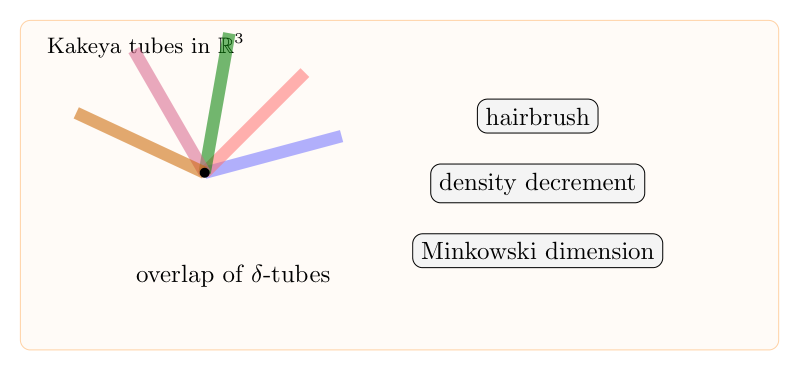
    this inequality is easy to proof.just observed that \mu(T_i\cap T_j)\sim \frac{1}{\theta_i-\theta_j}\delta^2.and to remember one thing:the inequality can be view as a uniformly estimate of overlap of the kakeya set,that is just mean the overlap would not concentrate to much at a lonely stick.this is enough to get a proof of the 2 dimension case just by a density decrement trick:we just not consider about the whole set I,but a low density subset \hat I\subset I,where \frac{|\hat I|}{|I|}\sim \delta^{\lambda},and make \lambda\to 0^+.

    Kakeya estimates

    Let \sigma\leq \delta\leq \theta<<1,and let T_{\delta} be a collection of \delta-tubes.whose set of directions all lie in a cap of radius \theta. Let 2<d<3 be fixed.
    • If we have a Kakeya estimate at some dimension d, and if the collection     T_{\delta} is direction-separated, then


    ||\sum_{i\in I}\chi_{T_i}||_{d'}\lesssim \delta^{\frac{d-3}{d}}\theta^{\frac{d+1}{d}}(1)
    • If we have an X-ray estimate at some dimension d, and if T_{\delta} consists ofessentially distinct tubes, then


     ||\sum_{i\in I}\chi_{T_i}||_{d'}\lesssim \delta^{\frac{d-3}{d}}\theta^{\frac{d+1}{d}}m^{1-\beta}
    for some β > 0, where m is the directional multiplicity of T_{\delta}.(2)

    So obviously the X-ray estimate is stronger than the kakeya estimate.it is just give the information of the overlap of the sticks with the same direction.

    in fact wolff have establish the X-ray estimate at dimension \frac{5}{2},so (2) just come from a rescaling argument.

    The sticky reduction

    renormalization process,just consider the process to make the thin sticks to be fat.and to proof this structure nearly has Markov property.but with a very small error term when change the scale.this is proved by the X-ray estimate.

    Triple intersection estimate

    Use Hardy-Litterwood-Soblev inequality,we can get a so called triple intersection estimate in general,said the triple intersection is smaller than the situation the 3 lines move together.and we just accosiate this to the cap-cup principle to get some information of the volume of X_{\delta}=\mu(\cup_{i\in I}T_i).img_0012

    Reduce to additive combination problem

    The right problem is just you have a n\times n cubes,and there is some sticks according them,if the distance of sticks is
    img_0011


    补充说明

    以下是新整理的中文说明;上方旧博客原文保持不变。

    Kakeya 猜想问:包含每个方向单位线段的集合是否必须有 full Hausdorff 或 Minkowski dimension?二维情形已经解决,三维情形则出现了 hairbrush、multiscale 和 sum-product 等深层结构。

    三维 Kakeya 猜想:hairbrush、密度递降与 Katz-Tao 思路
    三维 Kakeya 问题的困难来自不同方向细 tubes 的高重叠结构。

    1. Tube formulation

    令 $E_\delta$ 是 Kakeya set 的 $\delta$-neighborhood。Minkowski 维数问题等价于估计

    $$|E_\delta|\gtrsim_\varepsilon \delta^{\varepsilon}$$

    在合适维数归一化下的下界。更常用的语言是研究方向分离的 $\delta$-tubes 的重叠。

    2. 二维情形

    二维中,任意两个不同方向 tubes 的交叠容易控制。核心估计可以理解为:重叠不能集中在一根孤立 tube 附近。由此配合 density decrement,可推出二维 Kakeya 集合有 full dimension。

    3. Hairbrush 结构

    三维中,许多 tubes 可以围绕一根 tube 形成 hairbrush。Wolff 的观察是:如果很多 tubes 都与一根 tube 相交,那么它们的方向和位置仍然受到几何限制。这给出非平凡维数下界。

    4. Multiscale 难点

    Minkowski 版本比单尺度 maximal function 更微妙,因为不同尺度之间的结构会相互传递。一个尺度上的高重叠可能在下一尺度分裂,反过来又影响全局维数。

    5. Katz-Tao 方向

    Katz-Tao 的改进把 Kakeya 问题与 sum-product 现象联系起来。大致图像是:若 tubes 太集中,会诱导出同时具有加法和乘法结构的集合;sum-product 阻止这种集合太小。这是三维 Kakeya 后续发展的关键思想。

  • Fractal Uncertainty Principle:极限集、Schottky group 与 zeta 零点

    旧博客原文

    原题:Fractional uncertain principle

    semyon dyatlov的一篇文章

    semyon dyatlov的文章https://arxiv.org/pdf/1710.05430.pdf,用fractional uncertainly priciple导出了hyperbolic surface上测地线诱导的zeta函数在Re(s)>1-\epsilon只有有限个零点。


    就我的理解,这件事情至少和3个事情有关系,

    1.p-adic上的黎曼猜想,因为这篇文章的证明强烈依赖于markov性质,这和p adic的结构也很像,有可能可以利用p adic猜想的证明思路继续做一部分。


    2.billiard的传播子,但是这里不一样,文章中的 Schottky groups本质上是对于算子的逆写成一种级数形式其中级数由Schottky group生成,但是对于billiard传播子的情况所有的涉及的热核或者波核的paramatrix不仅仅具备markov性质,起主导作用的却是某种需要X-ray估计的性质,级数和并不是对全空间求而是某种截断了的子空间里面,所以比这个证明要难。建立起billiard的传播子估计是证明inverse spectral problem的重要一步。


    3.interval exchange map,但是interval exchange map的结构就好只有这里的traslation,这里有一个像的大小的指数衰减,这是interval exchange map所没有的。interval exchage map可能还需要涉及到一个拆分估计,会更难,这可能可以在interval exchange map上的sarnak猜想有进展。


    下面讲一下我对文章证明主要思路的理解:首先对于hyperbolic空间H^2/{\Gamma} 我们用poincare的方式来理解为 D mod掉一个作用,那么极限集\Lambda_{\Gamma} 就是基本域在分式线性变换下在D的边界下的极限点。

    关键是建立如下估计 \int_{\Lambda_{\Gamma}}exp (i\xi\phi(x)) g(x) d\mu(x)\leq C|\xi|^{−\epsilon_1} \forall \xi, |\xi| > 1.

    为了建立这个估计,我们做的事情是:

    1.研究极限集\Lambda_{\Gamma} 的结构,本质上具备某种组合上的树结构,在分式线性变换下树的上方和下方交换,而且对于象有指数级别的衰减,这很像连分数展开中的otrowoski表示。对于分式线性变换和Schottky group作用的体积形变估计是容易得到的。

    2.Patterson–Sullivan测度\mu 是在\Gamma 作用下的遍历测度,特别的,和 \Gamma 是compatible的,所以变量代换公式成立:

     \int_{\Lambda_{\Gamma}} f(x)d\mu(x) =\int_{\Lambda_{\Gamma}}f(\gamma(x))|\gamma'(x)|_{\delta}^B d\mu(x) \forall \gamma \in \Gamma

    这个很重要,一旦我们能够找到I :=\amalg_{b\in \Omega} I_b, 实际这可以导出一个关于f的方程:

     L_Zf(x) = \sum_{a\in Z,a\to b} f(\gamma_{a′}(x))w_{a′}(x), x ∈ I_b.

    我们关心的selberg zeta函数的零点就等于方程特征值1对应的特征函数: L_zf(x)=f(x) .

    (这一点很重要而且在很多问题中都有用,至少有几个例子:1.有的时候一个椭圆方程的特征值很难做,转而去考察他的发展方程。2.很多数论问题,特别是质数在某些partition集合里面的分布,对于对应的L函数的动力系统的刻画就需要这个方程)

    3. 文章中3.1.是bourgain的主要贡献,是所谓的sum-product现象在这里的一个引用,为了得到foriour衰减性估计,我们需要不断拆散区间,实际上在树的每一层上面我们都很清楚怎么把这一层的积分拆散到上一层和下一层,这实际上可以看成一个renormelization方程:

      \int_{\Lambda_{\Gamma}}f d\mu =\int_{\Lambda_{\Gamma}}L_{Z(\tau)}^{2k+1} f d\mu = \sum_{A,B,A\leftrightarrow B}f(\gamma_{A∗B}(x))w_{A∗B}(x)d\mu(x).

    1中的形变估计(只需要估计一下交叉项带来的误差)告诉我们:  | \int_{}fdμ|^2 ≤C\tau^{(2k−1)\delta}\sum_{A,B,A\leftrightarrow B} |\int_{I_b(A)} e^{iξ\phi(\gamma_{A∗B}(x))}w_{a′_k} (x)d\mu(x)| ^2 +C\tau^2 .

    然后在x点taylor展开用围道积分得到误差项,误差项用1中的形变估计得到上界控制,主项放到一起得到:

      |\int_{\Lambda_{\Gamma}} f d\mu|^2 ≤ C\tau^{(2k+1)\delta}\sum_A sup_{\eta\in J_{\tau}}| e^{2πi\eta\xi_{1,A} (b_1)···\xi_{k,A} (b_k )}| + C\tau^{\delta/4}. (*)

    最后为了用bourgain的sum-product现象得到的引理3.3来控制(*)RHS,我们需要对 R ⊂ Z(τ) ^{k+1} Z(τ)^{k+1}-R 分段估计,前者是用正则性导致的收敛速度快,后者shi用minkowki维数很小,前者估计已经建立,所以只需对Z(τ)^{k+1}-R 建立minkoski维数上界估计,这是显然的。

    这样我们就建立好了如下估计:

      \int_{\Lambda_{\Gamma}}exp ( i\xi\phi(x)) g(x) d\mu(x) ≤ C|\xi|^{−\epsilon_1} \forall \xi, |\xi| > 1.

    这个估计是用来建立fractional uncertain principle的关键,一旦我们有了fractional uncertain principle,hyperbolic surface上测地线诱导的zeta函数在Re(s)>\frac{1}{2}-epsilon只有有限个零点就只是一个fix point theorem的argument。

    另外一个不需要用sum-product现象的极为简单的证明见[1710.05430] Fractal uncertainty for transfer operators。


    补充说明

    以下是新整理的中文说明;上方旧博客原文保持不变。

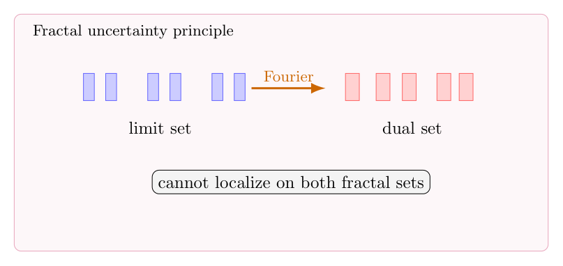
    Fractal uncertainty principle 说,一个函数不可能同时集中在一个 fractal set 和它的 Fourier dual fractal set 上。Dyatlov 等人的工作把这个原则用于 hyperbolic surface 上的共振和 Selberg zeta 函数零点问题。

    Fractal Uncertainty Principle:极限集、Schottky group 与 zeta 零点
    Fractal uncertainty principle 排除函数同时集中在极限集和对偶 fractal set 上。

    1. 从普通不确定性到 fractal 版本

    普通不确定性原理强调物理空间和频率空间不能同时局部化。fractal uncertainty principle 的形式更细:若 $X,Y$ 是具有 porous 或 Ahlfors-David regular 结构的 fractal sets,则不存在非零函数同时几乎支撑在 $X$ 和频率支撑在 $Y$ 上。

    粗略地说,有估计

    $$\|\mathbf 1_X \mathcal F_h \mathbf 1_Y\|_{L^2\to L^2}\le C h^\beta,$$

    其中 $\beta>0$ 反映 fractal 几何带来的额外衰减。

    2. Schottky group 与极限集

    对某些 hyperbolic surface,可以用 Schottky group 来描述。其极限集 $\Lambda$ 位于边界上,具有类似 Cantor set 的树状结构。群作用下的小区间长度指数衰减,而每一层的 cylinder 又保留清晰的组合编码。

    这和连分数、Ostrowski 表示、Markov partition 有相似味道:复杂轨道被编码成树上的路径,尺度之间通过 renormalization 关系联系。

    3. Patterson-Sullivan 测度

    Patterson-Sullivan 测度是极限集上的自然遍历测度。它与群作用兼容,因此变量替换公式可以把 transfer operator 写成适合迭代的形式。很多 zeta 函数或共振问题最终会转化为某个 transfer operator 是否有特征值 $1$。

    这一步很重要:谱问题从几何 Laplacian 转成边界动力系统上的算子问题。

    4. Sum-product 现象的作用

    fractal uncertainty 的关键估计往往来自 sum-product 型思想。若一个集合同时在加法和乘法结构上都太集中,就会违反 expansion。极限集的多尺度树结构让我们可以把振荡积分拆到不同层级,再用 expansion 迫使 Fourier 衰减。

    这与 Bourgain 方法的精神一致:不是直接逐点估计振荡积分,而是利用组合结构证明在多数尺度上不能同时对齐。

    5. 可能的延伸方向

    这个框架让人自然想到 billiards、interval exchange maps 和 $p$-adic 动力系统。相同点是都有编码和尺度结构;不同点是 Markov 性质、传播子 parametrix 和截断方式并不一样。真正困难的地方在于:如何找到一个既保留动力系统结构又能产生 Fourier 衰减的分解。

  • Fourier restriction problem 的自然性:从 Hausdorff-Young 到曲率

    旧博客原文

    原题:Natural of the restriction problem


    1.

    the most natural problem in harmonic analysis may be:

    investigate for what pair (p,q) we have :

    L^p(R^n)\longrightarrow L^q(R^n)

    \hat f(x)=\int_{R^n}e^{-2\pi ix\xi}f(\xi)d\xi

    is strong-(p,q) bounded.

    obvious we have the paserval identity:||\hat f||_{2}=||f||_2,and we have ||\hat f||_{\infty}\leq||f||_{1}.

    so by the Riesz-Thorin inteplotation theorem we have the Hausdorff-Young inequality:

    \forall 1\leq p\leq 2,\frac{1}{p}+\frac{1}{q}=1 we have:

    ||\hat f||_{q}\leq ||f||_{p}.

    now let talk about the rescaling trick:

    consider the transform:f(x)\longrightarrow f(\frac{x}{\lambda})=f_{\lambda}(x).we know if the inequality is right then it is necessary to have the same growth for the RHS and LHS.

    this argument will derive:\frac{n}{p}=n-\frac{n}{q}.

    in fact ||f_{\lambda}(x)||_{p}=\lambda^{\frac{n}{p}}||f(x)||_{p}.

    by the variable substitute formula:\hat f_{\lambda}(x)=\int_{R^n}e^{-2\pi ix\xi}f(\frac{\xi}{\lambda})d\xi=\lambda^n\hat f(\lambda x).

    so ||\hat f_{\lambda}(x)||_{q}=\lambda^{n-\frac{n}{q}}||\hat f(x)||_{q}

    and by the scaling invariance trick we know the pair (p,q) should live on the line \frac{1}{p}+\frac{1}{q}=1,and by test with the guessian function g(x)=e^{-x^2} we know the right pair  should be 1\leq p\leq 2.this end the problem with R^n.

    2.

    now replace R^n by a bounded open set K.when the fourior transform restriction on K is bounded p-q operator?

    i.e. L^p(R^n)\longrightarrow L^q(R^n)

    f\longrightarrow \hat f|_{K}.

    \hat f|_{K}=\int \chi_{K}e^{2\pi i<x,\xi>}f(\xi)d\xi.

    on a bounded set K,we always have:if q\geq r,||f||_{L^p(K)}\geq ||f||_{L^r(K)}.

    and associate with  hausdorff-young inequality we have:

    ||\hat f|_K||_{r}\leq ||\hat f||_q\leq ||f||_p.

    and this area is the exact area(rescaling trick and test with gaussian function),so end of the story.(but why?)

    3.

    Now we begin to deal with the really interesting case:K is not a open set but a sub manifold like the unit sphere S^{n-1}.

    ||\hat f||_{L^q(S^{n-1})}\leq ||f||_{L^p(R^{n})}.

    S^{n-1} equip with the usual surface measure \sigma.

    but the inequality is not always meaningful.

    case:p=2,\hat f\in L^2,in general can not restrict to a measure zero set due to the loss of regularity.

    case:p=1,\hat f continuous,meaningful to restrict to S^{n-1}.

    ||\hat f||_{L^{\infty}(S^{n-1})}\leq ||f||_{L^1(R^n)},\forall 1\leq p\leq \infty.

    Duality:we use the duality argument to transform the “restriction theorem” to “extension theorem”.

    T:f\longrightarrow \hat f.

    T:f\longrightarrow \hat f.

    ||f||=\sup_{||f||_p=1}||\hat f||_q=\sup_{||f||_p=1}\sup_{||g||_{q'}=1}|\int_{R^n}\hat fgd\sigma|=\sup_{||g||_{q'}=1}\sup_{||f||_p=1}|\int_{R^n}\hat fgd\sigma|=\sup_{||g||_{q'}=1}||\hat{gd\sigma}||_{p'}.

    4.

    we use R_s(p\to q) to state the estimate ||\hat f||_{L^q(S)}\leq ||f||_{L^p(R^n)}.S=S^{n-1}.

    and by rescaling argument we have natural condition:p<\frac{2n}{n-1},p'\geq \frac{n+1}{(n-1)q}.the restriction conjecture just say this necessary condition is also enough.

    Now we state the Tomas-Stein restriction theorem:

    1\leq p\leq \frac{2n+1}{n+3}.R_s(p\to 2) holds.

    this is the endpoint estimate in dimension 2 case,so by Meceztaze interpolation theorem this lead to the whole restriction theorem in dimension 2.

    the first argument is come from the so called TT^* trick that is find by fefferman and stein in 1970.

    T bdd p\to 2 \Longleftrightarrow TT^* bdd p'\to p.

    in fact:

    ||T||=\sup_{||f||_p=1}||Tf||_2=\sup_{||f||_p=1}\sup_{||g||_2=1}|\int (Tf)g|=\sup_{||f||_p=1}\sup_{||g||_2=1}|\int f(Tg)|=\sup_{||g||_2=1}||Tg||_{p'}=||T^*||.

    \int|e^{2\pi ix\xi}f(\xi)|^2 dw(\xi)\leq C||f||_p^2

    <\hat f,\hat fw(\xi)>\leq c||f||_p^2

    <\hat f,\hat{f*\hat{w(\xi)}}> \leq ||f||_p^2

    <f,f*\hat{w(\xi)}>\leq ||f||_p^2

    <f,f*\hat{w(\xi)}>\leq ||f||_p||f*\hat{w(\xi)}||_{p'}

    this can be derived from HLS inequality:

    ||f*\hat{w(\xi)}||_{p'}\leq ||f||_p.


    补充说明

    以下是新整理的中文说明;上方旧博客原文保持不变。

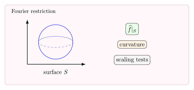
    restriction problem 问的是:Fourier transform 能不能有意义地限制到一个测度为零的曲面上?这件事在 $L^1$ 情形是平凡的,在一般 $L^p$ 情形却依赖曲面的曲率和振荡抵消。

    Fourier restriction problem 的自然性:从 Hausdorff-Young 到曲率
    restriction problem 的关键是把 Fourier transform 有意义地限制到带曲率的零测曲面上。

    1. 从 Hausdorff-Young 开始

    Fourier transform 满足 Plancherel

    $$\|\widehat f\|_2=\|f\|_2$$

    和显然估计

    $$\|\widehat f\|_\infty\le \|f\|_1.$$

    插值得到 Hausdorff-Young inequality:

    $$\|\widehat f\|_{p’}\le C\|f\|_p,\qquad 1\le p\le2.$$

    2. 为什么限制到曲面不平凡

    若 $S$ 是单位球面,想要估计

    $$\|\widehat f|_S\|_{L^q(S)}\le C\|f\|_{L^p(\mathbb R^n)}.$$

    因为 $S$ 是测度为零的集合,普通 $L^{p’}$ 控制不能直接给出 restriction。曲率让 Fourier transform 在曲面附近具有额外振荡结构。

    3. Scaling test

    任何 restriction estimate 必须通过 scaling 检验。用集中在小球或细 tube 上的 test functions,可以得到 $p,q$ 的必要关系。这些反例说明,restriction 问题不是纯函数分析问题,而是几何问题。

    4. Extension operator

    对偶形式是 extension estimate:

    $$Eg(x)=\int_S e^{ix\cdot\xi}g(\xi)\,d\sigma(\xi).$$

    它研究曲面上的振荡波如何在物理空间中叠加。曲率越强,波包方向越分散,越可能得到好的估计。

    5. 与 Kakeya 的联系

    restriction、Kakeya、Bochner-Riesz 和 wave packet decomposition 深度相连。曲面上的频率 cap 对应物理空间中的 tube;估计 extension operator 等价于控制这些 tubes 的重叠。

  • Kakeya 猜想的多尺度分析:旧 tubes、新 tubes 与密度递降

    旧博客原文

    原题:Kakeya Conjecture

    Last year I read a nice blog articles Recent progress on the Kakeya conjecture and have several questions with this article.

    follows the proof strategy called Multiscale analysis,although we can use the estimate with large \delta_1 to get estimate with small \delta_2,(may be loss some \delta^c in the inequality in this way),but the main difficult is we should proof the new tubes with scales \delta_2 is contains in the the olders.as soon as we proof this ,to obtain a lower bound of minkwoski dimension with kakeya set, suffice to get following estimate :
    the new cubes with scale \delta_2 contains a positive constants volumes of every old cubes with scale \delta_1.
    this type of estimate is easy to attain because it is very similar to the “principle of close packing of spheres”.

    in general ,we should not expect this claims:
    the new tubes with scales \delta_2 is contains in the the older.

    but if we can proof in some sense most of new tubes comes from this way maybe we can make progress on the original problem.

    roughly speaking,we should partition the whole set of T_{\delta} into two part,comes from old ones or not,for the first kind i.e contains in a old one,use the way explained above to treat.the second kind we need to proof the influence is very some or we can sometimes use the cubes from the first kind to instead the cubes from second kind and the measure of |A|_{\delta} change little.


    补充说明

    以下是新整理的中文说明;上方旧博客原文保持不变。

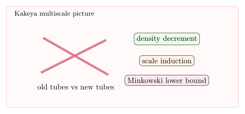
    Kakeya 猜想的多尺度分析试图把一个尺度上的 tube 结构传递到更小尺度。真正困难在于:新尺度上的 tubes 不一定整齐地包含在旧 tubes 中,必须区分继承结构和新出现结构。

    Kakeya 猜想的多尺度分析:旧 tubes、新 tubes 与密度递降
    Kakeya 多尺度分析的关键是判断小尺度 tubes 中哪些继承自旧尺度,哪些带来新结构。

    1. 多尺度想法

    设 $E_\delta$ 是 Kakeya set 的 $\delta$-neighborhood。若从尺度 $\delta$ 过渡到更小尺度 $\rho\delta$,希望旧尺度的每个有效 tube 都包含足够多的新尺度结构。

    2. 一个理想但错误的图像

    最天真的想法是:所有新 tubes 都来自旧 tubes 的细分。若如此,体积下界可以通过 close packing 直接传递。但实际情况中,新 tubes 可能跨越旧结构,产生新的重叠模式。

    3. 密度递降

    一种策略是把集合分成两类:继承旧结构的部分,以及真正新的部分。前者用尺度归纳处理;后者若太大,则会产生密度递降或结构性矛盾。

    4. 与 Katz-Tao 的关系

    Katz-Tao 方法中的 multiscale 思想正是利用尺度之间的结构约束。若某个尺度上 tubes 过度集中,会诱导出 additive/multiplicative 结构;sum-product 现象阻止这种结构无限持续。

    5. 关键问题

    多尺度方法的核心不是简单地把 tubes 变细,而是证明大部分新结构可以被旧结构解释;无法解释的部分必须带来额外 expansion。这个二分是 Kakeya 维数改进中的基本逻辑。