Remark 1 I thought this problem initial 5 years ago, cost me several days to find a answer, I definitely get something without the argument of Dirchlet hyperbola method and which is weaker but morally the same camparable with the result get by Dirichlet hyperbola method.
Remark 2 How to get the formula:
In fact,
Which is the integer lattices under or lying on the hyperbola .
Remark 3 By trivial argument, we can bound the quantity as following way,
The error term is , which is too big. But fortunately we can use the symmetry of hyperbola to improve the error term.
Proof:
Theorem 2
Given a natural number k, use the hyperbola method together
with induction and partial summation to show that
where denotes a polynomial of degree with leading term .
Remark 4 is the residue of at .
Proof:
We can establish the dimension 3 case directly, which is the following asymptotic formula,
The approach is following, we first observe that
The problem transform to get a asymptotic formula for the lattices under 3 dimension hyperbola. The first key point is, morally is the central point under the hyperbola.
Then we can divide the range into 3 parts, and try to get a asymptotic formula for each part then add them together. Assume we have:
.
.
.
Then the task transform to get a asymptotic formula,
But we can do the same thing for and then integral it. This end the proof. For general , the story is the same, by induction.
Induction on and use the Fubini theorem to calculate .
There is a major unsolved problem called Dirichlet divisor problem.
What is the error term? The conjecture is the error term is , it is known that is not right.
Remark 5
To beats this problem, need some tools in algebraic geometry.
2. Several problems
, is there a asymptotic formula for ?
, is a polynomial with degree , is there a asymptotic formula for ?
, is a polynomial with degree , is there a asymptotic formula for ?
Remark 6 In fact we can get , by combining the theorem 3 and 1.
3. Lattice points in ball
Gauss use the cube packing circle get a rough estimate,
In the same way one can obtain,
Remark 7 Where is the volume of the unit ball in dimension.
Dirchlet’s hyperbola method works nicely for the lattic points in a ball of dimension . Langrange proved that every natural number can be represented as the sum of four squares, i.e. , and Jacobi established the exact formula for the number of representations
Hence we derive,
This result extend easily for any , write as the additive convolution of and , i.e.
Apply the above result for and execute the summation over the remaining squares by integration.
Remark 8 Notice that this improve the formula 12 which was obtained by the method of packing with a unit square. The exponent in 16 is the best possible because the individual terms of summation can be as large as the error term (apart from ), indeed for we have if is odd by the Jacobi formula. The only case of the lattice point problem for a ball which is not yet solved (i.e. the best possible error terms are not yet established) are for the circle() and the sphere ().
Theorem 4
4. Application in finite fields
Suppose is a irreducible polynomial. And for each prime , let
By Langrange theorem we know . Is there a asymptotic formula for
A general version, we can naturally generated it to algebraic variety.
Is there a asymptotic formula for
Example 1 We give an example to observe what is involved. . We know is solvable iff or . One side is easy, just by Fermat little theorem, the other hand need Fermat descent procedure, which of course could be done by Willson theorem. In this case,
Which is a special case of Dirichlet prime theorem.
Let be an algebraic number field, i.e. the finite field extension of rational numbers, let
Dedekind proved that,
Theorem 5
is a ring, we call it the ring of integer of .
He showed further every non-zero ideal of could write as the product of prime ideal in uniquely.
the index of every non-zero ideal in is finite, i.e. , and we can define the norm induce by index.
Then the norm is a multiplication function in the space of ideal, i.e. .
Now he construct the Dedekind Riemann zeta function,
Now we consider the analog of the prime number theorem. Let , does the exist a asymptotic formula,
Given a prime , we may consider the prime ideal
Where is different prime ideal in . But the question is how to find these ? For the question, there is a satisfied answer.
Lemma 6 (existence of primitive element) There always exist a primetive elements in , such that,
Where is some algebraic number, which’s minor polynomial .
Theorem 7 (Dedekind recipe) Take the polynomial , factorize it in the polynomial ring ,
Consider . Then apart from finite many primes, we have,
Where .
Remark 9 The apart primes are those divide the discriminant.
Now we can argue that 4 is morally the same as counting the ideals whose norm is divide by in a certain algebraic number theory.
And we have following, which is just the version in algebraic number fields of 2.
Theorem 8 (Weber) of ideals of with norm equal to,
I explain some general ideal in the theory of diophantine approximation, some of them is original by myself, begin with a toy model, then consider the application on folklore Swirsing-Schmidt conjecture.
\tableofcontents
1. Dirichlet theorem, the toy model
The very basic theorem in the theory of Diophantine approximation is the well known Dirichlet approximation theorem, the statement is following.
Theorem 1 (Dirichlet theorem) for all is a irrational number, we have infinity rational number such that:
Remark 1 It is easy to see the condition of irrational is crucial. There is a best constant version of it, said, instead of , the best constant in the suitable sense for the theorem 1 should be and arrive by at least. The strategy of the proof of the best constant version involve the Frey sequences.
Now we begin to explain the strategies to attack the problem.
\paragraph{Argument 1, boxes principle} We begin with a easiest one, i.e. by the argument of box principle, the box principle is following,
Theorem 2 (Boxes principle) Given and two finite sets , set , if we have a map:
Then there exists a element such that there exist at least two element , .
Proof: The proof is trivial.
Now consider, , the sequences , then . Divide in an average way to part: . Then the linear structure involve (which, in fact play a crucial role in the approach). And the key point is to look at and integers.
\paragraph{Argument 2, continue fractional} We know, for irrational number , have a infinite long continue fractional:
Then
And we have,
Then .
\paragraph{Argument 3, Bohr set argument} We begin with some kind of Bohr set:
The key point is the shift of Bohr set, on the vertical line i.e. is very slow, and can be explained by
So:
in But in fact they are not really independent, as the number of Bohr sets increase, then you can calculate the correlation, thanks to the harmonic sires increasing very slowly, wwe can get something non trivial by this argument, but it seems not enough to cover the whole theorem 1.
\paragraph{Argument 4, mountain bootstrap argument} This argument is more clever than 3, although both two arguments try to gain the property we want in 1 from investigate the whole space but not , this argument is more clever.
Now I explain the main argument, it is nothing but sphere packing, with the set of balls
and define its subset
Then , and . If we can proof,
Lemma 3 For all , there is a subset of such that .
Remark 2 If we can proof 3, it is easy to see the theorem 1 follows.
Proof: The proof follows very standard in analysis, may be complex analysis? Key point is we start with a ball , whatever it is, this is not important, the important thing is we can take some ball with the center of in , then try to consider to extension and then we find the boudary is also larger then we can extension again, step by step just like mountain bootstrap argument. So we involve in two possible ending,
The extension process could extension to whole space.
we can not use the extension argument to extension to the whole space.
If we are in the first situation, then we are safe, there is nothing need proof. If we are in second case, anyway we take a ball . Then try to find good ball to approximate , but this is difficult…
Remark 3 Argument 1 is too clever to be true in generalization, argument 2 is standard, by the power of renormalization. argument 3 and argument 4 have gap… I remember I have got a proof similar to argument 4 here many years ago, but I forgot how to get it…
2. Schimidt conjecture
The Schimidt conjecture could be look as the generalization of Dirchlet approximation theorem 1 to algebraic number version, to do this, we need define the height of a algebraic number.
Definition 4 We say a number is a order algebraic number if and only is the minimal polynomial of , have degree .
Definition 5 (Height) Now we define the height of a th order algebraic number as , Where
Now we state the conjecture:
Theorem 6 (Swiring-Schimidt conjecture) For all transendental number , there is infinitely are th algebraic number such that:
Where is a constant only related to but not .
I point out the conjecture is very related to the map:
Where is the th symmetric sum.
Remark 4 is a map , what we consider is its inverse, , but is not smooth, it occur singularity when for some . And the map, as we know, the singularity depend on the quantity .
Remark 5 I then say something about the geometric behaviour of the map , as we know, what we have in mind is consider the map as a distortion , Then is just the pullback of the canonical metric on (morally) to .
高维 Diophantine approximation 会把一个数的逼近问题变成向量、线性形式或流形上的逼近问题。此时抽屉原理仍然给出基准结果,但最佳常数、例外集维数和代数数逼近会变得更深。许多问题最后会进入 geometry of numbers、dynamical systems on homogeneous spaces 或 Schmidt game 的语言。
First of all, we give the definition of discrete harmonic function.
Definition 1 (Discrete harmonic function) We say a function is a discrete harmonic function on if and only if for any , we have:
In dimension 2, the definition reduce to:
Definition 2 (Discrete harmonic function in ) We say a function is a discrete harmonic function on if and only if for any , we have:
The result establish in \cite{paper} is following:
Theorem 3 (Liouville theorem for discrete harmonic functions in ) Given . There exists a constant related to such that, given a discrete harmonic function in satisfied for any ball with radius , there is portion of points satisfied . then is a constant function in .
Remark 1 This type of result contradict to the intuition, at least there is no such result in . For example. the existence of poisson kernel and the example given in \cite{paper} explain the issue.
Remark 2 There are reasons to explain why there could not have a result in but in ,
The first reason is due to every radius there is only lattices in in so the mass could not concentrate very much in this setting.
The second one is due to there do not have infinite scale in but in .
The third one is the function in is automatically locally integrable.
The generation is following:
Theorem 4 (Liouville theorem for discrete harmonic functions in ) Given . There exists a constant related to such that, given a discrete harmonic function in satisfied for any ball with radius , there is portion of points satisfied . then is a constant function in .
In this note, I give a proof of 4, and explicit calculate a constant satisfied the condition in 3, this way could also calculate a constant satisfied 4. and point the constant calculate in this way is not optimal both in high dimension and 2 dimension.
2. some element properties with discrete harmonic function
We warm up with some naive property with discrete harmonic function. The behaviour of bad points could be controlled, just by isoperimetric inequality and maximum principle we have following result.
Definition 5 (Bad points) We divide points of into good part and bad part, good part is combine by all point such that , and is the residue one. So .
For all , we define for convenient.
Theorem 6 (The distribution of bad points) For all bad points in , they will divide into several connected part, i.e.
and every part satisfied .
Remark 3 We say is connected in iff there is a path in connected .
Remark 4 the meaning that every point So the behaviour of bad points are just like a tree structure given in the gragh.
Proof: A very naive observation is that for all is a connected compact domain, then there is a function
such that . And we have:
This could be proved by induction on the diameter if . Then, if there is a connected component of such that contradict to theorem 6 for simplify assume the connected component is just , then use the formula 5we know
The last line is due to consider around . But this lead to: which is contradict to the definition of . So we get the proof.
Now we begin another observation, that is the freedom of extension of discrete harmonic function in is limited.
Theorem 7 we can say something about the structure of harmonic function space of , the cube, you will see, if add one value, then you get every value, i.e. we know the generation space of
Proof: For two dimension case, the proof is directly induce by the graph. The case of dimensional is similar.
Remark 5 The generation space is well controlled. In fact is just like n orthogonal direction line in n dimensional case.
3. sktech of the proof for \ref
}
The proof is following, by looking at the following two different lemmas establish by two different ways, and get a contradiction.
\paragraph{First lemma}
Lemma 8 (Discrete poisson kernel) the poisson kernel in . We point out there is a discrete poisson kernel in , this is given by:
And the following properties is true:
, .
Remark 6 The proof could establish by central limit theorem, brown motion, see the material in the book of Stein \cite{stein}. The key point why this lemma 8 will be useful for the proof is due to this identity always true , So we will gain a lots of identity, These identity carry information which is contract by another argument.
\paragraph{Second lemma} The exponent decrease of mass.
Lemma 9 The mass decrease at least for exponent rate.
Remark 7 the proof reduce to a random walk result and a careful look at level set, reduce to the worst case by brunn-minkowski inequality or isoperimetry inequality.
\paragraph{Final argument} By looking at lemma 1 and lemma 2, we will get a contradiction by following way, first the value of on increasing too fast, exponent increasing by lemma2, but on the other hand, it lie in the integral expresion involve with poisson kernel, but the pertubation of poisson kernel is slow, polynomial rate in fact…
\newpage
{99} \bibitem{paper} A DISCRETE HARMONIC FUNCTION BOUNDED ON A LARGE PORTION OF Z2 IS CONSTANT
This is a note concentrate on the log average Sarnak conjecture, after the work of Matomaki and Raziwill on the estimate of multiplication function of short interval. Given a overview of the presented tools and method dealing with this conjectue.
1. Introduction
Sarnak conjecture \cite{Sarnak} assert that for any obersevable come from a determination systems , where , . The correlation of it and the Liuvillou function is 0, i.e. they are orthongonal to each other, more preseicesly it is just to say,
This is a very natural raised conjecture, Liuville function is the presentation of primes, due to we always believe the distribution of primes in should be randomness.
It has been known as observed by Landau \cite{Laudau} that the simplest case,
already equivalent to the prime number theorem. It is not difficult to deduce the spetial case of Sarnak conjecture when with the obersevation in $latex {(1)}&fg=000000$ come from finite dynamic system is equivalent to the prime number theorem in athremetic progress by the similar argument. Besides this two classical result, may be the first new result was established by Davenport,
Theorem 1 Let , is a inrational, then the obersevation come from is orthogonal to Mobius function. due to is a basis of , suffice to proof,
There is a lots of spetial situations of Sarnak’s conjecture have been established, The parts I mainly cared is the following:
Interval exchange map.
Skew product flow.
Obersevable come from One dimensional zero entropy flow.
Nilsequences.
But in this note, I do not want to explain the tecnical and tools to establish this result, but considering an equivalent conjecture of Sarnak conjecture, named Chowla conjecture, and explain the underlying insight of the suitable weak statement, i.e. the log average Chowla conjecture and the underlying insight of it.
The note is organized as following way, in the next section $latex {(2)}&fg=000000$, we give a self-contained introduction on the tools called Bourgain-Sarnak-Ziegler critation, explain the relationship of this critation and the sum-product phenomenon, also given some more general critation along the philosephy use in establish the Bourgain-Sarnak-Ziegler critation, which maybe useful in following development combine with some other tools. The key point is transform the sum from linear sum to bilinear sum and decomposition the bilinear sum into diagonal part and off-diagonal part, use the assume in the critation to argue the off-diagonal part is small and on the orther hand the diagonal part is also small by the trivial estimate and the volume of diogonal is small, this is very similar to a suitable Caderon-Zugmund decomposition.
In section $latex {(4)}&fg=000000$, I try to give a proof sketch of the result of Matomaki and Raziwill, which is also a key tools to understanding the Sarnak conjecture, or equivalent the Chowla conjecture. The key points of the proof contains following:
Find a suitable fourier indentity
Construct a multiplication-addition dense subset , and proof that the theorem MR hold we need only to proof it hold for instead of
Involve the power of euler product formula. divide the whole interval into a lot of small interval with smaller and smaller scale and a residue part. We look the part come from every small scale as a major term and look the residue part as minor term.
Deal with the major term at every scale, by a combitorios identity and second moments method.
find a enough decay estimate from a scale to the next smaller scale.
Deal with the minor term by the H… lemma.
Due to the theorem of MR do not exausted the method they developed, we trying to make some more result with their method, Tao and Matomaki attain the average version of Chowla conjecture is true by this way, and combine this argument and the entropy decresment argument they established the 2 partten of the log average Chowla conjecture is true. Very recently Tao and his coperator proved the odd partten case of log average chowla conjecture is true, combine an argument of frustenberg crresponding principle and entopy decresment argument. But it seems the even and large than 2 case is much difficult and seems need something new to combine with the method of MR and entropy decresment and frunstenberg corresponfing principle to make some progress.
So, in section $latex {(5)}&fg=000000$, we give a self-contain introduction to the entropy decresment argument of Tao, and combine with the frustenberg corresponding principle.
In the last section $latex {(6)}&fg=000000$, I state some result and method and phylosphy of them I get on nilsequences and wish to combine them with the previous method to make some progress on log average Chowla conjecture on the even partten case.
\newpage
2. Bourgain-Sarnak-Zieglar creation
We begin with the easiest one, this is the main result established in \cite{BSZ}, I try to give the main ideal under the proof, but with a no quantitative version is the following,
Theorem 2 (Bourgain-Sarnak-Zieglar creation, not quantitative version) if for all primes we have:
Then for multiplication function we have
Remark 1 For simplify we identify .
Remark 2
The idea is following, break the sum into a bilinear one, so, of course, we multiplication it with itself. i.e. we consider to control,
To control 4, we need exhausted the mutiplication property of , we have . We can not get good estimate for all term,
The condition in our hand if following,
So, just like the situation of Cotlar-Stein lemma \cite{Cotlar-Stein lemma}, we wish to estimate like following:
Then we consider divide the sum into diagonal part and non-diagonal part, as following,
But the first part is small, i.e.
Because of
and the second part is small, i.e.
Because diagonal part is small in and trivial inequality
But the method in remark 2 is not always make sense in any situation, we need to construct two suitable sets and then break up into , this mean,
But this could be construct in this situation, thanks to the prime number theorem,
Theorem 3 (Prime number theorem)
Morally speaking, this is the statement that the primes, which is the generator of multiplication function, is not very sparse.
3. Van der curpurt trick
There is the statement of Van der carport theorem:
Theorem 4 (Van der curpurt trick) Given a sequences in , if , is uniformly distributed, then is uniformly distributed.
I do not know how to establish this theorem with no extra condition, but this result is true at least for polynomial flow. \newpage Proof:
This type of trick could also establish the following result, which could be understand as a discretization of the Vinegradov lemma.
Remark 3
Uniformly distribution result of : Given , coverages to a uniformly distribution in as .
Remark 4 But I definitely do not know how to establish the similar result when .
Remark 5
This trick could also help to establish estimate of correlation of low complexity sequences and multiplicative function, such as result:
Maybe with the help of B-Z-S theorem.
\newpage
4. Matomaki and Raziwill’s work
In this section we explain the main idea underlying the paper \cite{KAISA MATOMA 虉KI AND MAKSYM RADZIWILL}. But play with a toy model, i.e. the corresponding corollary of the original result on Liouville鈥檚 function.
The most important beakgrouth of analytic number theory is the new understanding of multiplication function on share interval, this result is established by Kaisa Matom盲ki and Maksym Radziwill. Two very young and intelligent superstars.
The main theorem in them article is :
Theorem 6 (Matomaki,Radziwill) As soon as when , one has:
for almost all .
In my understanding of the result, the main strategy is:
Parseval indetity, transform to Dirchelet polynomial.
Involved by multiplication property, spectral decomposition.
From linear to multilinear , Cauchy schwarz inequality.
major term estimate.
Estimate the contribution of area which is not filled.
4.1. Parseval indetity, transform to Dirchelet polynomial
We wish to establish the equality,
This is the norm, by Chebyschev inequality, this could be control by norm, so we only need to establish the following,
We wish to transform from the discretization sum to a continue sum, that is,
Remark 7 There are two points to understand why 19 and 18 are the same.
Now we try to transform 19 by Parseval indetity, this is something about the norms of the quality we wish to charge. It is just trying to understanding 19 as a quantity in physical space by a more chargeable quality in frequency space. Image,
Then . Note that,
So by Parseval identity, we have,
Remark 8 We know the Fejer kernel satisfied,
So morally speaking, we get the following identity.
In fact we do a cutoff, the quality we really consider is just:
established the monotonically inequality:
Theorem 7 (Paserval type identity)
Remark 9
In my understanding, This is a perspective of the quality, due to the quality is a multiplicative function integral on a domain with additive structure, it could be looked as a lots of wave with the periodic given by primes, so we could do a orthogonal decomposition in the fractional space, try to prove the cutoff is a error term and we get such a monotonically inequality.
But at once we get the monotonically inequality, we could look it as a聽compactification process and this process still carry most of the information so lead to the inequality.
It seems something similar occur in the attack of the moments estimate of zeta function by the second author. And it is also could be looked as something similar to the 聽spectral decomposition with some basis come from multiplication generators, i.e. primes.
4.2. Involved by multiplication property, spectral decomposition
I called it is “spectral decomposition”, but this is not very exact. Anyway, the thing I want to say is that for multiplication function , we have Euler-product formula:
But anyway, we do not use the whole power of multiplication just use it on primes, i.e. leads to following result:
This is a identity about the function , the point is it is not just use the multiplication at a point,i.e. , but take average at a area which is natural generated and compatible with multiplication, this identity carry a lot of information of the multiplicative property. Which is crucial to get a good estimate for the quality we consider about.
4.3. From linear to multilinear , Cauchy schwarz
Now, we do not use one sets , but use several sets which is carefully chosen. And we do not consider [X,2X] with linear structure anymore , instead reconsider the decomposition:
On every it equipped with a bilinear structure. And is a very small set, which is in fact have much better estimate.
Now we just use a Cauchy-Schwarz:
4.4. major term estimate
4.5. estimate the contribution of area which is not filled
\newpage
5. Entropy dcrement argument
\newpage
6. Correlation with nilsequences
I wish to establish the following estimate: is the liouville function we wish the following estimate is true.
Where we have as ,
is a compact space.
I do not know how to prove this but this is result is valuable to consider, because by a Fourier identity we could transform the difficulty of (log average) Chowla conjecture to this type of result.
There is some clue to show this type of result could be true, the first one is the result established by Matomaki and Raziwill in 2015:
Theorem 8 (multiplication function in short interval)
is a multiplicative function, i.e. . as , then we have the following result,
And there also exists the result which could be established by Vinagrodov estimate and B-S-Z critation :
Theorem 9 (correlation of multiplication function and nil-sequences in long interval)
is a multiplicative function, i.e. . is a polynomial function then we have the following result,
\newpage {9} \bibitem{Sarnak} Peter Sarnak, Mobius Randomness and Dynamics.
\texttt{https://publications.ias.edu/sites/default/files/Mahler }. \bibitem{Laudau} JA 虂NOS PINTZ (BUDAPEST). LANDAU鈥橲 PROBLEMS ON PRIMES.
\texttt{https://users.renyi.hu/~pintz/pjapr.pdf} \bibitem{BSZ} Knuth: Computers and Typesetting,
The story of the infinite dimensional space of $\Delta$ is following, we eliminate ourself with compact smooth non-boundary manifold $M$ with metric $g$, then we have Betrami-Laplace operator $\Delta_g$. We could instead $\Delta_g$ by hodge laplace $dd^*+d^*d$, but let we consider $\Delta_g$ the eigenvalue problem:
$$\Delta_g u=\lambda u$$
A classical way to investigate the eigenvalue problem is according to consider variational principle and max-min principle. We equip the path integral on the function space $C^{\infty}(M)$:
$$E(f)=\frac{\int_M |\nabla u|^2}{\int_M |u|^2 }$$
Then it have a sequences of eigenvalue, negative of course: $$0<-\lambda_1<-\lambda_2<…<\lambda_k<…$$
Then things become interesting, the morse theory of infinite space involve, called the infinite space as $X$, so at least, shrink the far place of $X$ as a point, in physics, this mean, cut off at fix scale. And we can take the scale to infinite small, we use the cutoff one to approximation the real one. What I can do is the following, I can proof the eigenvalue function is uniformly distributed in $L^2(M_g)$ (after rescaling of course) and the classical weyl law(although can not give a good error term estimate), but thing become more complicated when I try to consider the infinite space $X_{M_g}$’s topology, at finite scale at least, i.e. $X_{M_g}^{h}$ which is the cut off at scale $h$. Among the other thing, I believe the following issue is true, but without ability to proof it:
>**Problem**
for every manifold $M$ and metric $g$ on $M$, the topology of infinite space $X_{M_g}$ is the same, beside this, the inverse could be true, i.e. If $X_{M_1},X_{M_2}$ is not homomorphism for some scale $h$ then $M_1,M_2$ is not homomorphism.
By intuition, I think it is depend by the underling manifold’s topology. But I do not have a rigorous proof, I definitely have a non-rigorous one, if ignore the coverage…
As I find this problem when I try to give a proof of weyl law, I do not check the reference, may be this problem is a classical one? As always, I will appreciate to any interesting comments and answers, thanks a lots!A
2.
We begin with our favorite situation, the Dirchlet problem on bounded simple-connected domain $\Omega$ in $\mathbb R^n$. Let $\lambda_1$ be the first eigenvalue of $$\Delta u=\lambda u \ in\ \Omega$$
$$u=0\ \ on\ \partial\Omega$$
Rescaling $u$ such that $\sup_{\Omega} u=1$, I think the following property of the first eigenvalue is true.
>**Problem**
We have, the Minkowski functional of $\Omega$, called $M_{\Omega}$ and the Minkowski functional with the ball $B$ such that $vol(B)=vol(\Omega)$, then along the level set of $u$, i.e. the fiber: $$\Omega=\cup_{t\in [0,1]}l_t, l_t:=\{t|x\in \Omega, u(x)=t\}$$
We pretend for the isolate point $l_1$ to be a ball with radius 0, so equipped it with the uniformly density at every direction in $S^1$, i.e. the mass distribution given by $M_B$ and the total mass coincide with the total mass induce by $M_{\Omega}$ in $l_0$, i.e.
$$\int_{e\in S_1}M_{\Omega}(e)d\mu=\int_{e\in S_1}M_{B}(e)d\mu$$
The measure $d\mu$ equipped on $S^1$ is the natural Haar measure. And the cost function is given by $c(x,y)=\|x-y\|^2$. Then, among this setting,
I wish the following property to be true:
Along the direction $1\to 0$, the transport of density $\partial_{t_0} M_{\cup_{t=t_0}^1l_t}$ given the unique optimal transport of the natural measure induce by $M(\Omega)$ and $M(B)$.
**Remark 1** As point out by SebastianGoette, the multiplicity of the first eigenvalue must be one, thanks to the eigenfunction never change the symbol, so we are in the best case.
**Remark 2**:I am not very sure this property could always true, there may be a center example when $\Omega$ is not convex, but I tend to believe it is true at least when $\Omega$ is convex.
**Remark 3**: As point out by Dirk, when you try to consider the optimal transport problem, you always need to point out the cost function $c(x,y)$ defined on $\Omega \times \Omega$, for there, I think the naive choice is $c(x,y)=\|x-y\|^2$
The thing I can proof is the following, the level set of $u$ should be convex by brunn-minkowski inequality, and some type of monotonically property, i.e. more and more like a ball when the level set is more and more shirking smaller form $\partial \Omega$ to the point $f$ arrive maximum.
I will appreciate for any relevant comments and answer, thanks!
Is there a Brunn-Minkowski inequality approach to the phenomenon charged by uncertainty principle? More precisely, is it possible to say some thing about the Gaussian distribution
to be the best choice that arrive minimum?
Remark 1 Or some other suitable distance space on reasonable function (may be some gromov hausdorff distance? Any way, to say the guassian distribution is the best function to defect the influence of uncertain principle.
I do not know the answer of the problem 1, but this is a phenomenon of a universal phylosphy, aid, uncertainty principle, heuristic:
It is not possible for both function and its Foriour transform to be localized on small set.
Now let me give some approach by intuition to explain why the phenomenon of “uncertainty principle” could happen.
The approach is based on:
level set decomposition.
area formula (or coarea formula), anyway, some kind of change variable formula.
integral by part.
Basic understanding on exponential sum.
Let our function the Shwarz space, we begin with a intuition (not very rigorous) calculate:
Now we try to understanding the result of the calculate, it is,
The calculate is wrong, but not very far from the thing that is true, the key point is now the exponential sum involve. We could use the pole coordinate in the frequence space and get some very rough intuition of why the the uncertainty principle could occur.
Remark 2 Why we consider the level set decomposition, due to the integral is a combination of linear sum of the integral on every level set, so shape of level set is the key point.
The part of in 2 is a rotation on the level set, a wave correlation of it and the christization function of level set in the whole space, this is of course a exponential sum.
Now we can begin the final intuition explain of the phenomenon of uncertainty principle. If the density of function is very focus on some small part of the physics space, then it is the case for level sets of , but we could say some thing for the exponential sum 3 related to the level set, just by very simply argument with hardy litterwood circle method or Persaval identity? Any way, something similar to this argument will make sense, due to if the diameter of level set focus ois small, then we can not get a decay estimate for when along one direction in frequency space, in fact we could say the inverse, i.e. it could not decay very fast.
2. Bernstein’s bound and Heisenberg uncertainty principle
2.1. Motivation and Bernstein’s bound
There is two different Bernstein’s bound, we discuss the first with the motivation, and proof the second rigorously. \paragraph{Form 1} is a invertible affine map, then for a ball , is a ellipsoid.
By a orthogonal transform we could make to be a diagonal matrix, i.e. . It is said, for or is a smooth bump function, , so we have,
We define dual of , .
Remark 3 Why there we use the metric but not the standard inner product ? How to understand the choice?
Proposition 1 We have the following property:
.
Remark 4
This is a norm of related to .
Proof: Suffice to proof 2.
More quantitative we have rigorous one: \paragraph{Form 2} If , , then it is not possible for to be concentrate on a scale much less than .
Proof: case is trivial by Paserval identity, which said on , fourier transform is a isometry, . For general case, integral by part, and use trivial estimate,
2.2. Heisenberg inequality
Theorem 3 (Heisenberg uncertain principle), so , . then for any , every direction, we have
Remark 5 We could understand the inequality by the following way. suffice to prove it with and then by approximation argument. , define . then we have the following:
Remark 6 The inequality is shape, the extremizers being precisely given by the modulated Gaussians: arbitrary
There are two proof strategies I have tried, I try them for several hour but not work out with a satisfied answer, the method more involve, I explain what happen in section 1, I have not tried, I will try it later. Both this two strategies i face some difficulties, I explain why I can not work out them with a proof: \paragraph{Strategy 1} The first one is, we could work with of course, by approximation, then we find, by Paserval, and are both true. then we use our favourite way to use Cauchy-Schwarz, the difficulty is we can not use a integral by part argument directly, even after restrict ourselves with monotonic radical symmetry inequality and by a rearrangement inequality argument, it seems reasonable due to rearrangement decreasing the kinetic energy as said in Lieb’s book. But even work with monotonic one, then one involve with some complicated form, try to use Fubini theorem to rechange the order of integral try to say something, it is possible to work out by this way but I do not know how to do. There is some calculate under this way,
but you know, at a point we have , the reasonable calculate is following,
We want , Then
Seems to be … I do not know.
\paragraph{Strategy 2} The second strategy is, in the quantity we lose two cone very near , we need use the extra thing to make up them. May be effective argument come from some geometric inequality.
3. The Amerein-Berthier theorem
Next we investigate following problem, the problem is following: if are of finite measure, can there be a nonzero with and ? Some argument is folowing: Observe that:
Assume that: then . So we have, at least . Some dirty calculate show:
So we can define kernel of ,
By Fubini, we calculate the Hilbert-Schmidt norm:
So is a compact operator and its operator norm satisfied . So if then we can canculate we can not have in the original question.
The story is in fact more interesting, the answer of the question is no even for , so in all case. We have the following quatitative theorem:
Theorem 4 finite measure in , then
for some constant .
Remark 7 There is a naive approach for this theorem: Area formula trick, the shape of level set. Obvioudly we have:
Key point is proof:
Let us do some useless further calculate:
So suffice to have:
But there is connter example given by modified scaling Gaussian distribution… The point is form 15 to 16 is too loose.
Following I given a right approach, following by my sprite on level set and area formula argument and discritization.
Proof: The story is the same for a discretization one. We need point out, change the space to , then every thing become a discretization one, and the change could been argue as a approximation way. What happen then, we have a naive picture in mind which is:
What is the case with norm, it become the standard nner product on , and the scale involve, i.e. we have the following basic estimate:
Now image if the density of concentrate in a very small area, then by a cut off argument we consider the supp of , is very small, then use the argument 18, we could conclute the density of could not very concentrate in the fraquence space. The constant could be given presicely by this way, but I do not care about it.
4. Logvinenko-Sereda theorem
Next we formulate some result that provide further evidence of the non-concentration property of functions with Fourier support on .
4.1. A toy model
Theorem 5 Let an suppose that satisfies,
If satisfies then
Where as .
Proof: This is a easy corollary of the argument I give in the proof of Amerein-Berthier theorem 4.
4.2. A refine version
Theorem 6 Suppose that a measurable set satisfies the following “thinkness” condition: there exists such that
where is arbitrary but fixed. Assume that . Then
where the constant depends only on and .
Remark 8 This proof need some very good estimate come from several complex variables.
5. The Malgrange-Ehrenpreis theorem
Theorem 7 Let be a bounded domain in and let be a polynomial, Then, for all , there exists such that in a distribution sence.
In this short note, I posed a conjecture on Brunn-Minkwoski inequality and explain why we could be interested in this inequality, what is it meaning for further developing of some fully nonlinear elliptic equation come from geometry. The main part of the note devoted to discuss several different proof of classical Brunn-Minkowski inequality.
I believe, every type of Brunn-Minkowski inequality, type of Brunn-Minkowski inequality is in some special sense and will be explained later, will be crucial with a corresponding regularity result of a fully nonlinear elliptic equation which could be realizable by geometric way which will also explained in further note.
So the key point is that Brunn-Minkowski inequality is crucial and have potential application, I posed a problem there and then consider the classical Brunn-Minkowski inequality, we give several proof of the classical Brunn-Minkowski inequality, everyone could help us to have a more refine understanding of the original difficulty with different angle.
Theorem 1 (conjecture) We have a map
We are willing to called the function as the hamiltonian function. then we could consider the hamiltonian flow of the function , but this could only true for a even dimension manifold to make there exists that is a non-degenerate closed form.
Anyway we consider the level set of , we get a foliation i.e . we consider the gradient flow with , called the gradient flow begin with as . And we wish the gradient flow have a addition structure on itself then we could consider what is the Brunn-Minkowski inequality in this setting, the condition is a group structure on the space of level set , i.e.
Remark 1 take in 1, this conjecture reduce to the toy model, i.e. classical Brunn-Minkowski inequality.
Remark 2 We could generate the problem to the problem which is charged by several energy function , if the induced gradient flow is amenable, then this is somewhat similar with the one dimension case, I wish if we could do something for the single function , then we can say something for the several functions involved case.
Remark 3 This could also generate to amenable group action case and quantization of it.
Meaning, the cohomology induce by a hamiltonian system on some special foliation on fiber of geometric bundle. This type of result could help to establish the vanish of the cohomology, the get the existence theory and regularity result for corresponding elliptic nonlinear differential equation. And solve the original problem I consider.
Now we given the statement of Brunn-Minkowski inequality.
Theorem 2 (brunn minkowski inequality) For measurale set in . we have following,
“>
The general spproach of Brunn-Minkwoski inequality is following,
divide the measurable set into small cubes.
Shinking trick, transform the set into convex one.
for the first one, we have the following lemma,
Lemma 3, measurable set, , , and , and
Proof: The proof of the lemma is a easy corollary of the construction of Lesbegue(or Borel) measurable algebra.
Remark 4 The existence of the property given in the lemma is not the key point, the key point is .
Has this two simplify in hand, we could give several approach to proof the inequality and these proof carry information more than just a proof, they carry some information with the structure of space . \newpage
2. A proof with discretization
There is a lots of ways to attack the Brunn-Minkowski inequality, the most natural one is discretization. But unfortunately there is some technique obstacle for proof or even state the discretization version of “Brunn-Minkowski” inequality.
The “boundary” and “area” should not compatible.
And we need use the fact,
Now we just state what we expect it should transform in, because we have a fully understanding with the discretization model, there is a result named Cauchy-Daveport inequality.
Theorem 4 (cauchy-daveport inequality) There are two case, one in , one in finite field .
case, are finite set,we have,
case, are finite set,we have,
Proof: for the case, the story is more or less trivial, just do to a observation, if , then
There exists a strictly increasing chain of length at least .
For the case, following is a graph to explain what happen, basically we define a operation on tuples, i.e. , and make the additive energy decreasing. after induction with this transform and the transform from a tuple to the minimum additive energy by translation, the additive energy decreasing and decreasing then arrive the global minimum. But it is easy to conclude in this case one of become null set and then the inequality 8 follows.
But when we discrete the Brunn-Minkowski inequality, we expect a high dimension generation of the inequality 4. Naively we wish,
Theorem 5 (naive generation of cauchy-daveport inequality) For , and are finite sets,
But this is not the case, there is a counterexample for 5. We could construct some such that , consider they be very thin line.
So why we are in this worse situation? because we lose the information of , . So they have the trend tending to make the “boundary” campatible with “area”. Two thin line in the same direction is exactly the worst case, which is just a equal condition of 1-dimension case.
One natural way to except the situation is to bounded the “isperimetric constant”, to assume varies in a subset of measurable set, with addition condition that is bounded by some constant. But this is also not the suitable set for our inequality, I explain how to capture the information of the G-H coverage.
Now assume are convex bounded set, and we take a global orthogonal basis in . named . We give the definition of discretization of , named .
Definition 6 ( discretization) The construction of from is following:
divide into , is the cubes.
use or instead of depending on iff , where is a given number only rely on . i.e.
glue them, define .
Now we describe the condition of rigorous meaning campatible with discretization.
Under the basis, there is a coordinate we could know iff is the cube center at if it is in . Due to is convex, is lipchitz. So you will have some locolization property, said, at every fix discretization scale , the position of is morally known so the number of cubes in in the one dimensional affine space which is the subspace of the number is asymptopic to the dimensional hausdorff measure of . So at least,
Property 11 is crucial, which mean is really a n-dimensional space and automatically we have the bounded on isoperimetric constant .
Now we can look at every and take limit . In fact we a in the situation with Accumulation of wood to make the product have smallest volume. Not to optimized the tuples but fix one of it, said , optimized the other one, said . This is the key point of proof, a little bit different from the argument of dimensional 4 where we optimized the tuple.
Key point:
we can ignore “small core”.
This inequality is said, due to , the convex of the functional on convex set.
The way of discretization could not handle the problem but definitely said that the difficulty occur with the shape of boundaries .
3. A proof with “central of mass” and Minkowski functional
Definition 7 (Central of mass) The central of mass of measurable set , if exist, satisfied, , there is a subspace with codimension 1 divide into two connected part such that
then .
Remark 5 For a measurable set , if central of mass exists, then there exist only one. This is a easy observation do to the definition of , i.e. the intersection of suitable affine subspace in every direction.
Theorem 8 (existence of central of mass)
Proof: It is easy to attain by take different directions in , then easy to proof every line across it be definition of .
Definition 9 (Minkowski functional) for a measurable set and a point , define on , such that
.
Remark 6 If is convex, then is a convex function on , so it is lipchitz.
we have following formula for the measure of .
Theorem 10
Proof: trivial.
Now the task reduce fixing and to optimized make small. It is the same as make small when fix and . Due to
This approach is a nonstandard one, due to I believe the renormlization or continue fractional or multilinear estimate is everywhere. We first play with a toy model, the rectangle.
Theorem 11 Brunn-Minkowski inequality is right for are rectangles.
5. connection of Brunn-Minkowski inequality and Sobolev inequality, the firth proof
We begin with a calculate based on intuition and it is not rigorous.
The second line is due to I believe there such that it is a equality, by the equal condition of Minkowski inequality, in fact this is morally inverse of Minkowski inequality. The second reason in general case why the second inequality is true is due to a rescaling argument, change , by the rescaling argument we conclude if there is a such inequality, the index of it must be the case.
原题:Pesudo differential opertor and singular integral
I already understand this material 3days ago but it is a little difficult for me to type the latex…
1. Introduction
There is two space to understand a function’s behaviour, the physics space and the frequency space (Why thing going like this? Why there is such a duality?). Namely, we have:
The key point is, waves is a parameter group of scaling of definition of a constant fraquence wave, so it connected the multiplication and addition. Basically due to it can be look as the correlation of a function and the scaling of wave with carry all the information about . A generation of this obeservation is the wavelet theory.
So as we well know, the key ingredient of Fourier transform is to image function as a sum of series waves. A famous theorem of Mikhlion said that a translation-invariant operator on could be represented by a multiplication operator on the Fourier transform side. translation is the meaning, is a translation.
In a formal level, consider it as distribution (compact distribution or temperature distribution is both OK). We have:
the meaning is if we consider is a operator on distribution space, , then ,
due to the linear combination of will consititue a dense set in . So this could extend to the whole distribution space by dual and give the definition of , i.e.
Remark 1 is bounded on when is a bounded function, thanks to Parevel theorem. When is a bounded function, the composition of two such operator could be defined, and the symbol of composition operator corresponding to the composite of their symbol, i.e.
Remark 2 For parenval theorem, i.e. , there is two approach, heat kernel approximation approach and discretization.
We wish to investigate the operator given by multiplier, i.e.
When it is satisfied ?
Intuition, the following calculate is only morally true, not rigorous.
So we need some restriction on , namely , so we need some decay condition on , why this, just consider integral by part for . The rigorozaton of this intuition inspirit us to the definition of symbol calss.
Definition 1 we say is in symbol class iff,
for all is multi-indece.
Remark 3
we note that all partial differential operator, whose coefficient, together with all their derivatives are bounded belong to this class, In this particular circumstance, the symbol is a polynomial in , essentially the “characteristic polynomial” of the operator.
The general operator of this class have a parallel description in terms of their kernels. That is, in a suitable sense,
besides enjoying a cancellation property, is here characterized by differential inequalities “dual” to those for . In the key case where the order , this kernel representation makes a singular integral operator.
The crucial estimate, when , is atelatively simple consequences of Plancherel’s theorem for the Fourier transform. With this, the theory introduce in previous note is therefore applicable.
The product identity that holds in the translation-invariant case generalized to the situation treated here as a symbolic calculus for the composition of operators. That is, there is an asymptotic formula for the composition of two such operators, whose main term is the point-wise product of their symbols.
The succeeding terms of the formula are of decreasing orders. These orders measure not only the size of the symbols, but determine also the increasing smoothing properties of the corresponding operators. The smoothing properties are most neatly expressed in terms of the Sobolev space and the Lipschitz space .
2. Pseudo-differential operator
“Freezing principle”: from variable coefficient differential equation to constant coefficient differential equation by approximation. divide into 2 steps:
divide space into small cubes.
take average of the coefficient of differential equation in every cubes.
Suppose we are interested in study the solution of the classical elliptic second order equation.
Where the coefficient matrix is assume to be real, symmetric, positive definite and smooth in . Understanding , such that,
Looking for a . Such that . is a error term which have good control. To do this, fix an arbituary point , freeze the operator at :
In Fourier sense ( sence).
Remark 4 The remark is, morally speaking, for application of fourier transform in PDE. morally we could only solve the problem with linear differential equation (although we could consider the hyperbolic type). The main obstacle for Fourier transform application into PDE:
it only make sense with Schwarz class or its dual, this is not main obstacle, in principle could be solved by rescaling.
the main obstacle is it only compatible with linear differential equation.
Cut-off function: vanish near the origin,
then:
is actually a smoothing operator, because it is given by convolution with a fixed test function. It should be seasonable when near , is well approximated by , it is actually the case, define , i.e.
The operator so given is a propotype of a pesudo-differential operator. Moreover, one has , where the error operator is “smoothing of order 1”. That this is indeed the case is the main part of the symbolic calculus described.
Definition 2(symbol class) A function belong to and is said to be of order of is a function of and satisfies the differential inequality:
For all are multi-indece.
Now we trun to the exact meaning of pesudo-differential operator, i.e. how them action on functions. Under some suffice given regularity condition, for , .
Remark 5 is continuous and for pointwise, , in .
then expense it, we get:
This could be diverge, even when . The key point is we do not have control with the second integral, morally speaking, this phenomenon is the weakness of Lesbegue integral which would not happen in Riemann integral, so sometime we need the idea from Riemann integral, this phnomenon is settle by multi a cut off function and take , the same deal also occur as the introduced of P.V. integral in Hilbert transform. The precise method to deal with the obstacle is following: , if , . in the sense:
, ,
We also have:
Then we have:
and denotes . Thus the pesudo-differential operator initially defined as a mapping from to , extend via the identity 17 to a mapping from the space of temperatured distribution to itself . Notice also that is automatically continuous in this space. \newpage
3. bounded theorem
We first introduce a powerful tools, called dyadic decomposition,
Lemma 3(dyadic decomposition) In eculid space there exists a function such that,
and , there is only two of such that , and we can choose to be radical and .
Remark 6
So for a given mutiplier , we will have .
Proof: The proof is easy, after rescaling we just need observed there is a bump function satisfied whole condition.
Theorem 4 Suppose is a symbol of order 0, i.e. that Then the operator , initially defined on , extends to a bounded operator from to itself.
Remark 7 Suffice to show and by dual.
In fact we can directly proof a more general theorem:
Theorem 5 Let satisfy, for any multi-index of length ,
For all . Then, for any , there is a constant such that,
for all .
Proof:, so we have:
are multi indeces. Then we consider dyadic decomposition, the is a function satisfied the condition in 19, define . then cpt, . So , we have,
have good decay estimate, thanks to , this estimate is deduce morally along the same ingredient of “station phase”, it is come from a argument combine “counting point” argument and a rescaling argument. So,
But we have , ending the proof.
Remark 8 this method also make sense of restrict the condition to be:
Where is the dimension of the space, and we could change to .
Remark 9
is a counter example for .
Remark 10 The key point is the estimate
Correlation of taylor expension and wavelet expension. This is also crutial for the theory of station phase.
4. Calculus of symbols
This calculus of symbols would imply there is some structure on this set.
Theorem 6 Suppose are symbols belonging to and respectively. Then there is a symbol in so that:
Moreover,
in the sense that,
For all .
The following “proof” is not rigorous, we just calculate it formally, we could believe it is true rigorously, by some approximation process. Proof: We assume have compact support so that our manipulations are justified. We use the alternate formula 15 to write,
Then we apply , again in the form 15, but here with the variable replacing in the integration. The result is,
This calculate is easy to derive, but the following is more tricky. Now , so
with
we can also carry out the integration in the y-variable. This leads to the corresponding Fourier transform of in that variable, and allows us to rewrite 30 as,
With this form in hand, use taylor expense to the symbol , i.e.
with a suitable error term , due to
we only need to proof and it is definitely the case, we get the theorem.
Remark 11 We need replace with , where
we note that satisfy the same differential inequalities that and do, uniformly in .passage to the limit as will then give us our desired result.
5. Estimate in , Sobolev, and Lipchitz space
We now take up the regularity properties of our pesudo-differential operator as expressed in terms of the standard function spaces, we begin with the boundedness of an operator of order .
5.1. estimate
Suppose belongs to the symbol class . Then, we can express as
due to , we know, with some approximation argument and first do it with a cutoff symbol of , i.e. , that,
So that the integral coverage whenever and is away from the support of . Since we know that is bounded on , this representation extends to all for almost every . More generally, we have,
hence satisfies,
Use the general singular integral theory we get the following estimate.
Theorem 7 Suppose is the pseudo-differential operator corresponding to a symbol in , then extends to a bounded operator on to itself, for .
5.2. Sobolev spaces
We first recall the definition of the Sobolev spaces , where is a positive integer. A function belongs to if and the partial derivatives , taken in the sense of distribution, belong to , whenever . The norm in is given by,
the following result is the directly corollary of 7.
Theorem 8 Suppose is a pseudo-differential operator whose symbol belongs to . If is an integer and , then is a bounded mapping from to , whenever .
Remark 12 This theorem remain valid for arbitrary real .
5.3. Lipschitz spaces
Theorem 9 Suppose is a symbol in . Then the operator is a bounded mapping from to , whenever .
Lemma 10 Suppose the symbol belongs to , and define . Then, as operator from to itself, the have norms that satisfy
We shall now point out a very simple but useful alternative characterization of . This is in terms of approximation by smooth functions; it is also closely connected with the definition of space as intermediate spaces, using the “real” method of interpolation.
Corollary 11 A function belongs to if and only if there is a decomposition,
with , for all , where is the smallest integer .
When , the argument prove 10, with , , gives the required estimate for the .
This is the first note of a series of notes concert on semiclassical analysis. Given the basic material on symplectic geometry. Including the following material,
The case at a point, or we can look it as the case in .
The standard material in symplectic geometry, i.e. Hamiltonian mechanics, two approach, global one concentrating on lie derivative, and a locally one concentrating on the power of Darboux theorem, i.e. the existence of a canonical coordinate.
The basic facts on Poission bracket.
The basic facts on Lagrange sub-manifold, and the involve of Liouville measure.
2. Case of a point, or
Let be a vector field, at once we have a vector field, we could consider the associated flow of it,
express the trajectory start from along the vector field.
Remark 1 There . One the other hand, due to the locally existence theorem of ODE, if the regularity of is enough, then the solution exist and is uniqueness.
Definition 1 or more convenient . We call the flow map or the exponential map generated by .
Lemma 2 For flow map, we have following:
for all .
for all .
for each time , the mapping is a diffeomorphism with
So it is a group action on , with units as diffeomorphism of . Proof:
This lemma is the direct corollary of the theory of ODE.
Now let us special to the case . In local coordinate we have , express position of particle, express momentum of particle.
Definition 3 in define their symplectic product,
In a matrix form, coincide with a matrix
Following lemma given the basic property of .
Lemma 4 The following basic property are true.
,
the bilinear form is antisymmetric, and degenerate, i.e. if for all , then .
, .
Proof:
trivial calculate get this.
trivial.
, by basic linear algebra everything follows.
3. Hamiltonian mechanics
Definition 5 Symplectic form: non-degenerate closed 2 form in a standard coordinate(Darboux coordinate, coordinate like ) looks like,
, map
is an isomorphism. is called the symplectic form.
There is locally coordinate for , i.e.,
So , roughly we have , this is of course not true, but morally true. Now let us give the definition of symplectic manifold and the relationship of Hamiltonian mechanics.
Definition 6 We have the following definition,
A symplectic manifold is a pair where is a smooth manifold and is a closed two-form on such that the map,
is an isomorphism, is called the symplectic form.
If is symplectic, and is differentiable, the hamiltonian vector field of is the field on whose image under the previous map is . In other word, is characticed by the property,
The flow of will be referenced to as the hamiltonian flow of .
Lemma 7 If coordinate and the symplectic form
then,
If is differentiable, then the integral curves of are the solutions to the system of ODEs,
Moreover, if
Where is a smooth solution (“potential”), and is a trajectory of the Hamiltonian flow of , then
This is the Newton’s second law for the force .
Proof:, due to we have . So we have:
Assume . Then we have,
and also,
Combine with the definition of integral curve we derive the integral curves of i.e. such that , is given by 5.
Now we begin to proof the Newton second law for the force . We consider the 2-dimensional case at first. We have,
The high dimension case is similar, thanks to the linearity of and .
Remark 2 Two make Newton’s second law to be true, the form 6 play a crucial role. Is there some generalization of this type of result to more general case, roughly speaking, it is reasonable to expect this could still be true if the hamiltonian function could be divide into potential energy part and kinetic energy part. And the describe of potential energy part is that it is given by a quadratic form.
Lemma 8 In general, for any Hamilton field one has:
, conservation of energy. In orther word, is everywhere tangent to the level sets of .
, so the Hamiltonian flow of consists of automorphism of .
General speaking, to proof a theorem on manifold, there always have two choice, coordinate free proof and proof in a careful choose coordinate. If we choose to believe the Darboux theorem 9 is true, the meaning of it is that locally the symplectic manifold are the same.
Proof: If we believe the Darboux theorem 9 is true. then consider in a standard coordinate , we have,
So of course . In general case, i.e. coordinate free proof, . Use identity if lie derivative. The second thing is also easy to proof by look in a local canonical coordinate, involve the indentity of lie derivative.
Remark 3 I need more understanding on the lie derivative, see wiki.
Theorem 9(Darboux theorem) Near any point there exist coordinate: usually called Darboux coordinates, such that the sympletic form has the form,
Remark 4 This theorem means there do not exist local invariant in symplectic manifold.
Proof:
\newpage
Theorem 10 If is any smooth manifold, then its cotangent bundle has a natural symplectic structure.
Proof: we have local coordinate on derive from , it is . Remember we have Riemann metric: on , the existence of Riemann metric involve a unit decomposition argument and bump function, I just recall it there. Now we move on, consider the relationship between .
Remark 5 It need not be the case that non-degenerate non-degenerate. This case in the lemma is a example to show that could be the case: degenerate non-degenerate. We glue something together on the space pf differential operator to understand the topology of it but not deifferential structure or more refinement structure. Quntalization could be look as a way to glue, this could be down if there is a differential equation with some special condition (come from a flow take charge of it suffice).
Lemma 11(The proof of is non-degenerate) Let be local coordinates on . Define a coordinate system on by the condition:
Prove that in Darboux coordinate, and therefore .
Proof:
Theorem 12 Let be a smooth Riemann manifold and let be one half of the square of the Riemann norm, so that in local coordinate,
Then the trajectorics of the hamiltonian flow of , projected down to , are geodesic aries in this fashion.
Newton’s second law+ energy vanish.
Proof:
So second variation formula describe of geodesic give us the fact that the trajective is geodesic.
Remark 6 We could directly calculate in local coordinate.
4. Poisson brackets
is the Hamiltonian generating the dynamic is any smooth function on phase space (the symplectic manifold), then the rate of change of along the trajectraries of d is the function
Definition 13 If is symplectic and , the poisson bracket of and is defined to be the function on .
Lemma 14 In canonical (Darboux) coordinate where , one has,
In particular, .
Proof:
Theorem 15 If is a symplectic manifold then is a Lie algebra.
Proof: Bilinearty, skew-symmetric come form,
Jacobi identity:
could be proved by calculate under a local coordinate.
There are some interesting problem, I post them at there in case I forget them. Excuse me if they are trivial, I have not took enough time to consider them about I think they are valuable to be consider.
Problem 1:
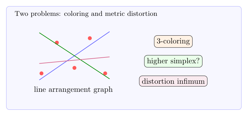
This problem is stated by graph coloring. there are two prat of it, in fact the first part I heard from someone else and I try to generate it to high dimension.
there are finite lines , crossing each other and the is a set of crossing point. for technique reason, assume the position of lines are generic, i.e. no three of them intersect at one point. Then we could use 3 different colors to color make Neighbor points have different color. And to proof 3 is smallest.
generate it to high dimension, to prove case, is the number.
This seems to be a graph problem, but the underlying structure is linear structure and some topological obstacle. I am not very sure. But it seems we can use an energy decrement argument with the obesevation:
The existence of a reasonable definition of “energy of correlation”.
the simplex arrive with the maximum of “correlation energy” in a very symmetric way, and this situation is easy to handle (coloring).
If make sense, this argument could also generate to high dimension.
Problem 2:
Let us consider some example of map between two metric space, a toy model is a line and two parallel lines, I called two parallel lines by , the single line by . The problem is try to find a tuple , where is a metric define on and . such that the distortion of and the standard metric on arrive at a infimum, this of course could not be the case, such like the situation of Yamabe problem on manifold with conners. So, let us ask a more general problem, could we describe the behavior of in some sense? what could we say with this kind of ?
![\displaystyle \sum_{1\leq n\leq x}d(n)=\sum_{1\leq n\leq x}[\frac{x}{n}]=xlogx+(2\gamma-1) x+O(\sqrt{x}) \ \ \ \ \ (1)](https://s0.wp.com/latex.php?latex=%5Cdisplaystyle+%5Csum_%7B1%5Cleq+n%5Cleq+x%7Dd%28n%29%3D%5Csum_%7B1%5Cleq+n%5Cleq+x%7D%5B%5Cfrac%7Bx%7D%7Bn%7D%5D%3Dxlogx%2B%282%5Cgamma-1%29+x%2BO%28%5Csqrt%7Bx%7D%29+%5C+%5C+%5C+%5C+%5C+%281%29&bg=ffffff&fg=000000&s=0&c=20201002)
.
![\displaystyle \sum_{1\leq n\leq x}d(x)=\sum_{1\leq n\leq x}[\frac{x}{n}]? \ \ \ \ \ (2)](https://s0.wp.com/latex.php?latex=%5Cdisplaystyle+%5Csum_%7B1%5Cleq+n%5Cleq+x%7Dd%28x%29%3D%5Csum_%7B1%5Cleq+n%5Cleq+x%7D%5B%5Cfrac%7Bx%7D%7Bn%7D%5D%3F+%5C+%5C+%5C+%5C+%5C+%282%29&bg=ffffff&fg=000000&s=0&c=20201002)
![\displaystyle \sum_{1\leq n\leq x}d(x)=\sum_{1\leq ab\leq x}1=\sum_{1\leq n\leq x}[\frac{x}{n}]\ \ \ \ \ (3)](https://s0.wp.com/latex.php?latex=%5Cdisplaystyle+%5Csum_%7B1%5Cleq+n%5Cleq+x%7Dd%28x%29%3D%5Csum_%7B1%5Cleq+ab%5Cleq+x%7D1%3D%5Csum_%7B1%5Cleq+n%5Cleq+x%7D%5B%5Cfrac%7Bx%7D%7Bn%7D%5D%5C+%5C+%5C+%5C+%5C+%283%29&bg=ffffff&fg=000000&s=0&c=20201002)
, which is too big. But fortunately we can use the symmetry of hyperbola to improve the error term.
![\displaystyle \begin{array}{rcl} \sum_{1\leq n\leq x}[\frac{x}{n}] & = & \sum_{1\leq ab\leq x}1\\ & = & x\sum_{i=1}^x\frac{1}{i}-\sum_{i=1}^x\{\frac{x}{i}\}\\ & = &xlnx+\gamma x+O(x) \end{array}](https://s0.wp.com/latex.php?latex=%5Cdisplaystyle+%5Cbegin%7Barray%7D%7Brcl%7D+%5Csum_%7B1%5Cleq+n%5Cleq+x%7D%5B%5Cfrac%7Bx%7D%7Bn%7D%5D+%26+%3D+%26+%5Csum_%7B1%5Cleq+ab%5Cleq+x%7D1%5C%5C+%26+%3D+%26+x%5Csum_%7Bi%3D1%7D%5Ex%5Cfrac%7B1%7D%7Bi%7D-%5Csum_%7Bi%3D1%7D%5Ex%5C%7B%5Cfrac%7Bx%7D%7Bi%7D%5C%7D%5C%5C+%26+%3D+%26xlnx%2B%5Cgamma+x%2BO%28x%29+%5Cend%7Barray%7D+&bg=ffffff&fg=000000&s=0&c=20201002)
![\displaystyle \begin{array}{rcl} \sum_{1\leq n\leq x}d(n) & = & \sum_{ab\leq x}1\\ & = & \sum_{a\geq \sqrt{x}}[\frac{x}{b}]+\sum_{b\geq \sqrt{x}}[\frac{x}{a}]-\sum_{1\leq a,b\leq \sqrt{x}}1\\ & = & xlogx+(2\gamma-1)x+O(\sqrt{x}) \end{array}](https://s0.wp.com/latex.php?latex=%5Cdisplaystyle+%5Cbegin%7Barray%7D%7Brcl%7D+%5Csum_%7B1%5Cleq+n%5Cleq+x%7Dd%28n%29+%26+%3D+%26+%5Csum_%7Bab%5Cleq+x%7D1%5C%5C+%26+%3D+%26+%5Csum_%7Ba%5Cgeq+%5Csqrt%7Bx%7D%7D%5B%5Cfrac%7Bx%7D%7Bb%7D%5D%2B%5Csum_%7Bb%5Cgeq+%5Csqrt%7Bx%7D%7D%5B%5Cfrac%7Bx%7D%7Ba%7D%5D-%5Csum_%7B1%5Cleq+a%2Cb%5Cleq+%5Csqrt%7Bx%7D%7D1%5C%5C+%26+%3D+%26+xlogx%2B%282%5Cgamma-1%29x%2BO%28%5Csqrt%7Bx%7D%29+%5Cend%7Barray%7D+&bg=ffffff&fg=000000&s=0&c=20201002)


denotes a polynomial of degree
with leading term
.

is the residue of
at
.
![\displaystyle \sum_{1\leq xy\leq n}[\frac{n}{xy}]=xP_2(logx)+O(x^{1-\frac{1}{3}+\epsilon}) \ \ \ \ \ (5)](https://s0.wp.com/latex.php?latex=%5Cdisplaystyle+%5Csum_%7B1%5Cleq+xy%5Cleq+n%7D%5B%5Cfrac%7Bn%7D%7Bxy%7D%5D%3DxP_2%28logx%29%2BO%28x%5E%7B1-%5Cfrac%7B1%7D%7B3%7D%2B%5Cepsilon%7D%29+%5C+%5C+%5C+%5C+%5C+%285%29&bg=ffffff&fg=000000&s=0&c=20201002)
![\displaystyle \sum_{1\leq xy\leq n}[\frac{n}{xy}]=\sum_{xyz\leq n}1 \ \ \ \ \ (6)](https://s0.wp.com/latex.php?latex=%5Cdisplaystyle+%5Csum_%7B1%5Cleq+xy%5Cleq+n%7D%5B%5Cfrac%7Bn%7D%7Bxy%7D%5D%3D%5Csum_%7Bxyz%5Cleq+n%7D1+%5C+%5C+%5C+%5C+%5C+%286%29&bg=ffffff&fg=000000&s=0&c=20201002)
![{([n^{\frac{1}{3}}],[n^{\frac{1}{3}}],[n^{\frac{1}{3}}])}](https://s0.wp.com/latex.php?latex=%7B%28%5Bn%5E%7B%5Cfrac%7B1%7D%7B3%7D%7D%5D%2C%5Bn%5E%7B%5Cfrac%7B1%7D%7B3%7D%7D%5D%2C%5Bn%5E%7B%5Cfrac%7B1%7D%7B3%7D%7D%5D%29%7D&bg=ffffff&fg=000000&s=0&c=20201002)
.
.
.

![{\sum_{1\leq yz\leq [n^{\frac{2}{3}}]}[\frac{r}{yz}]}](https://s0.wp.com/latex.php?latex=%7B%5Csum_%7B1%5Cleq+yz%5Cleq+%5Bn%5E%7B%5Cfrac%7B2%7D%7B3%7D%7D%5D%7D%5B%5Cfrac%7Br%7D%7Byz%7D%5D%7D&bg=ffffff&fg=000000&s=0&c=20201002)


![\displaystyle \begin{array}{rcl} \frac{\{\frac{kn}{1}\}+\{\frac{kn}{2}\}+...+\{\frac{kn}{n}\}}{n} & = & \frac{\sum_{i=1}^k\frac{kn}{i}-\sum_{i=1}^n[\frac{kn}{i}]}{n}\\ & = & k(lnn+\gamma +\epsilon_n)-\frac{\sum_{i=1}^{kn}[\frac{kn}{i}]-\sum_{i=n+1}^{kn}[\frac{kn}{i}]}{n} \end{array}](https://s0.wp.com/latex.php?latex=%5Cdisplaystyle+%5Cbegin%7Barray%7D%7Brcl%7D+%5Cfrac%7B%5C%7B%5Cfrac%7Bkn%7D%7B1%7D%5C%7D%2B%5C%7B%5Cfrac%7Bkn%7D%7B2%7D%5C%7D%2B...%2B%5C%7B%5Cfrac%7Bkn%7D%7Bn%7D%5C%7D%7D%7Bn%7D+%26+%3D+%26+%5Cfrac%7B%5Csum_%7Bi%3D1%7D%5Ek%5Cfrac%7Bkn%7D%7Bi%7D-%5Csum_%7Bi%3D1%7D%5En%5B%5Cfrac%7Bkn%7D%7Bi%7D%5D%7D%7Bn%7D%5C%5C+%26+%3D+%26+k%28lnn%2B%5Cgamma+%2B%5Cepsilon_n%29-%5Cfrac%7B%5Csum_%7Bi%3D1%7D%5E%7Bkn%7D%5B%5Cfrac%7Bkn%7D%7Bi%7D%5D-%5Csum_%7Bi%3Dn%2B1%7D%5E%7Bkn%7D%5B%5Cfrac%7Bkn%7D%7Bi%7D%5D%7D%7Bn%7D+%5Cend%7Barray%7D+&bg=ffffff&fg=000000&s=0&c=20201002)
![\displaystyle S_k(n)=\sum_{i=1}^{kn}[\frac{kn}{i}]-\sum_{i=n+1}^{kn}[\frac{kn}{i}] \ \ \ \ \ (10)](https://s0.wp.com/latex.php?latex=%5Cdisplaystyle+S_k%28n%29%3D%5Csum_%7Bi%3D1%7D%5E%7Bkn%7D%5B%5Cfrac%7Bkn%7D%7Bi%7D%5D-%5Csum_%7Bi%3Dn%2B1%7D%5E%7Bkn%7D%5B%5Cfrac%7Bkn%7D%7Bi%7D%5D+%5C+%5C+%5C+%5C+%5C+%2810%29&bg=ffffff&fg=000000&s=0&c=20201002)
![\displaystyle \begin{array}{rcl} S_k(n) & = & (2\sum_{i=1}^{[\sqrt{kn}]}[\frac{kn}{i}]-[\sqrt{kn}]^2)-(\sum_{i=1}^k[\frac{kn}{i}]-kn)\\ & = & 2\sum_{i=1}^{[\sqrt{kn}]}\frac{kn}{i}-\sum_{i=1}^k\frac{kn}{i}+2\{\sqrt{kn}\}[\sqrt{kn}]+\{\sqrt{kn}\}^2-2\sum_{i=1}^{[\sqrt{kn}]}\{\frac{kn}{i}\}+\sum_{i=1}^k\{\frac{kn}{i}\}\\ & = & 2kn(ln[\sqrt{kn}]+\gamma+\epsilon_{[\sqrt{kn}]})-kn\sum_{i=1}^k\frac{1}{i}+r(n)\\ & = & knln(kn)+kn(2\gamma-\sum_{i=1}^k\frac{1}{i})+r'(n)\\ & = & knln n+kn(2\gamma+lnk-\sum_{i=1}^k\frac{1}{i})+r'(n) \end{array}](https://s0.wp.com/latex.php?latex=%5Cdisplaystyle+%5Cbegin%7Barray%7D%7Brcl%7D+S_k%28n%29+%26+%3D+%26+%282%5Csum_%7Bi%3D1%7D%5E%7B%5B%5Csqrt%7Bkn%7D%5D%7D%5B%5Cfrac%7Bkn%7D%7Bi%7D%5D-%5B%5Csqrt%7Bkn%7D%5D%5E2%29-%28%5Csum_%7Bi%3D1%7D%5Ek%5B%5Cfrac%7Bkn%7D%7Bi%7D%5D-kn%29%5C%5C+%26+%3D+%26+2%5Csum_%7Bi%3D1%7D%5E%7B%5B%5Csqrt%7Bkn%7D%5D%7D%5Cfrac%7Bkn%7D%7Bi%7D-%5Csum_%7Bi%3D1%7D%5Ek%5Cfrac%7Bkn%7D%7Bi%7D%2B2%5C%7B%5Csqrt%7Bkn%7D%5C%7D%5B%5Csqrt%7Bkn%7D%5D%2B%5C%7B%5Csqrt%7Bkn%7D%5C%7D%5E2-2%5Csum_%7Bi%3D1%7D%5E%7B%5B%5Csqrt%7Bkn%7D%5D%7D%5C%7B%5Cfrac%7Bkn%7D%7Bi%7D%5C%7D%2B%5Csum_%7Bi%3D1%7D%5Ek%5C%7B%5Cfrac%7Bkn%7D%7Bi%7D%5C%7D%5C%5C+%26+%3D+%26+2kn%28ln%5B%5Csqrt%7Bkn%7D%5D%2B%5Cgamma%2B%5Cepsilon_%7B%5B%5Csqrt%7Bkn%7D%5D%7D%29-kn%5Csum_%7Bi%3D1%7D%5Ek%5Cfrac%7B1%7D%7Bi%7D%2Br%28n%29%5C%5C+%26+%3D+%26+knln%28kn%29%2Bkn%282%5Cgamma-%5Csum_%7Bi%3D1%7D%5Ek%5Cfrac%7B1%7D%7Bi%7D%29%2Br%27%28n%29%5C%5C+%26+%3D+%26+knln+n%2Bkn%282%5Cgamma%2Blnk-%5Csum_%7Bi%3D1%7D%5Ek%5Cfrac%7B1%7D%7Bi%7D%29%2Br%27%28n%29+%5Cend%7Barray%7D+&bg=ffffff&fg=000000&s=0&c=20201002)


, by combining the theorem 3 and 1.


is the volume of the unit ball in


in 16 is the best possible because the individual terms of summation can be as large as the error term (apart from
), indeed for
we have
if
is odd by the Jacobi formula. The only case of the lattice point problem for a ball which is not yet solved (i.e. the best possible error terms are not yet established) are for the circle(
) and the sphere (
).

![{f(x)\in {\mathbb Z}[x]}](https://s0.wp.com/latex.php?latex=%7Bf%28x%29%5Cin+%7B%5Cmathbb+Z%7D%5Bx%5D%7D&bg=ffffff&fg=000000&s=0&c=20201002)






. We know
is solvable iff
or
. One side is easy, just by Fermat little theorem, the other hand need Fermat descent procedure, which of course could be done by Willson theorem. In this case,


![\displaystyle \mathcal{O}_K=\{\alpha\in K, \alpha \ satisfied \ a\ monic \ polynomial\ in\ {\mathbb Z}[x]\} \ \ \ \ \ (23)](https://s0.wp.com/latex.php?latex=%5Cdisplaystyle+%5Cmathcal%7BO%7D_K%3D%5C%7B%5Calpha%5Cin+K%2C+%5Calpha+%5C+satisfied+%5C+a%5C+monic+%5C+polynomial%5C+in%5C+%7B%5Cmathbb+Z%7D%5Bx%5D%5C%7D+%5C+%5C+%5C+%5C+%5C+%2823%29&bg=ffffff&fg=000000&s=0&c=20201002)
is a ring, we call it the ring of integer of
uniquely.
in
, and we can define the norm induce by index.
.
![\displaystyle N(I):=[\mathcal{O}_K:I] \ \ \ \ \ (24)](https://s0.wp.com/latex.php?latex=%5Cdisplaystyle+N%28I%29%3A%3D%5B%5Cmathcal%7BO%7D_K%3AI%5D+%5C+%5C+%5C+%5C+%5C+%2824%29&bg=ffffff&fg=000000&s=0&c=20201002)


is some algebraic number, which’s minor polynomial

, factorize it in the polynomial ring
,
. Then apart from finite many primes, we have,
.


of ideals of
equal to,
![\displaystyle \rho_k(X)+O(x^{1-\frac{1}{d}}), where \ d=[K:Q] \ \ \ \ \ (31)](https://s0.wp.com/latex.php?latex=%5Cdisplaystyle+%5Crho_k%28X%29%2BO%28x%5E%7B1-%5Cfrac%7B1%7D%7Bd%7D%7D%29%2C+where+%5C+d%3D%5BK%3AQ%5D+%5C+%5C+%5C+%5C+%5C+%2831%29&bg=ffffff&fg=000000&s=0&c=20201002)
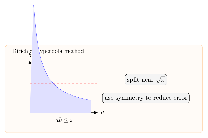
 is a irrational number, we have infinity rational number
  such that: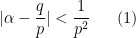
 , the best constant in the suitable sense for the theorem
  and arrive by
  at least. The strategy of the proof of the best constant version involve the Frey sequences.
  and two finite sets
  , set
, set  , if we have a map:
 such that there exist at least two element
  ,
,  .
. , the sequences
  , then
 ![{\{ix\}\in [0,1], \forall i\in \{1,2,...,n\}}](https://s0.wp.com/latex.php?latex=%7B%5C%7Bix%5C%7D%5Cin+%5B0%2C1%5D%2C+%5Cforall+i%5Cin+%5C%7B1%2C2%2C...%2Cn%5C%7D%7D&bg=ffffff&fg=000000&s=0&c=20201002) . Divide
. Divide ![{[0,1]}](https://s0.wp.com/latex.php?latex=%7B%5B0%2C1%5D%7D&bg=ffffff&fg=000000&s=0&c=20201002) in an average way to
in an average way to  part:
part: ![{[\frac{k-1}{N},\frac{k}{N}]}](https://s0.wp.com/latex.php?latex=%7B%5B%5Cfrac%7Bk-1%7D%7BN%7D%2C%5Cfrac%7Bk%7D%7BN%7D%5D%7D&bg=ffffff&fg=000000&s=0&c=20201002) . Then the linear structure involve (which, in fact play a crucial role in the approach). And the key point is to look at
. Then the linear structure involve (which, in fact play a crucial role in the approach). And the key point is to look at  and integers.
 ,
, 


 .
.
 is very slow, and can be explained by

 But in fact they are not really independent, as the number of Bohr sets increase, then you can calculate the correlation, thanks to the harmonic sires increasing very slowly, wwe can get something non trivial by this argument, but it seems not enough to cover the whole theorem

 , and
, and  . If we can proof,
 , there is a subset
  of
of  such that
 ![{\cup_{i\in A_l}B_i=[0,1]}](https://s0.wp.com/latex.php?latex=%7B%5Ccup_%7Bi%5Cin+A_l%7DB_i%3D%5B0%2C1%5D%7D&bg=ffffff&fg=000000&s=0&c=20201002) .
.  , whatever it is, this is not important, the important thing is we can take some ball
  with the center of
  to extension
  to whole space.
 . Then try to find good ball
  is a
is a  order algebraic number if and only is the minimal polynomial of
  have degree
 ![{deg(f)=n, f\in {\mathbb Z}[x]}](https://s0.wp.com/latex.php?latex=%7Bdeg%28f%29%3Dn%2C+f%5Cin+%7B%5Cmathbb+Z%7D%5Bx%5D%7D&bg=ffffff&fg=000000&s=0&c=20201002) .
.  , Where
 , there is infinitely
 is a constant only related to
 is the
  is a map
  , what we consider is its inverse,
  , but
, but  is not smooth, it occur singularity when
  for some
  . And the map, as we know, the singularity depend on the quantity
  .
.  is just the pullback of the canonical metric on
  (morally) to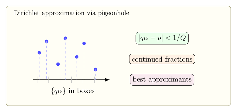
 is a discrete harmonic function on
  if and only if for any
  , we have:
 )
)  is a discrete harmonic function on
  if and only if for any
  , we have:
 . There exists a constant
  related to
  such that, given a discrete harmonic function
  in
in  with radius
  , there is
  portion of points
  satisfied
  . then
  there is only
  lattices in
  in
in  )
)  . There exists a constant
  such that, given a discrete harmonic function
  satisfied the condition in
  satisfied
  is the residue one. So
  .
. , we define
  for convenient.
 in
in 
 satisfied
  .
. is connected in
  .
.  is a connected compact domain, then there is a function
 . And we have:
 . Then, if there is a connected component of
 . But this lead to:
  which is contradict to the definition of
  , the cube, you will see, if add one value, then you get every value, i.e. we know the generation space of
 ,
,  .
.
 , So we will gain a lots of identity, These identity carry information which is contract by another argument.
  increasing too fast, exponent increasing by lemma2, but on the other hand, it lie in the integral expresion involve with poisson kernel, but the pertubation of poisson kernel is slow, polynomial rate in fact…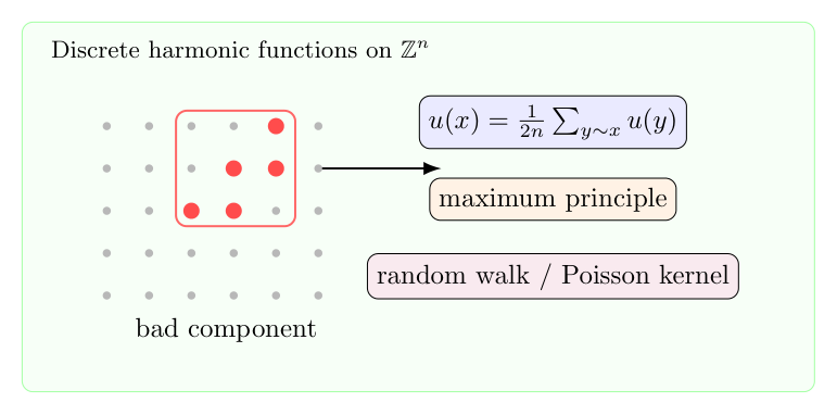
 come from a determination systems
  , where
  ,
,  . The correlation of it and the Liuvillou function is 0, i.e. they are orthongonal to each other, more preseicesly it is just to say,
 should be randomness.
 ,
,  is orthogonal to Mobius function. due to
  is a basis of
  , suffice to proof,
 , and proof that the theorem MR hold we need only to proof it hold for
 ![{S\cap [1,2,...,n]}](https://s0.wp.com/latex.php?latex=%7BS%5Ccap+%5B1%2C2%2C...%2Cn%5D%7D&bg=ffffff&fg=000000&s=0&c=20201002) instead of
instead of ![{[1,2,...,n]}](https://s0.wp.com/latex.php?latex=%7B%5B1%2C2%2C...%2Cn%5D%7D&bg=ffffff&fg=000000&s=0&c=20201002)
 we have:
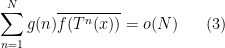
 .
. 
 . We can not get good estimate for all term,

![\displaystyle \begin{array}{rcl} |\sum_{p\in W}\sum_{n\in V}F(pn)g(pn)| & \leq & \sum_{n\in V}|g(n)|\cdot |\sum_{p\in W}F(pn)g(p)| \\ & \leq &\sum_{n\in V}|\sum_{p \in W}F(pn)g(p)|\\ & \overset{Cauchy-Schwarz}\leq & |V|^{\frac{1}{2}}[\sum_{n\in V}|\sum_{p\in W}F(pn)g(p)|^2]^{\frac{1}{2}}\\ & = & |V|^{\frac{1}{2}}[\sum_{p_1,p_2\in W}\sum_{n\in V}F(p_1n)\overline{F(p_2n)}g(p_1)\overline{g(p_2)}]^{\frac{1}{2}}\\ \end{array}](https://s0.wp.com/latex.php?latex=%5Cdisplaystyle+%5Cbegin%7Barray%7D%7Brcl%7D+%7C%5Csum_%7Bp%5Cin+W%7D%5Csum_%7Bn%5Cin+V%7DF%28pn%29g%28pn%29%7C+%26+%5Cleq+%26+%5Csum_%7Bn%5Cin+V%7D%7Cg%28n%29%7C%5Ccdot+%7C%5Csum_%7Bp%5Cin+W%7DF%28pn%29g%28p%29%7C+%5C%5C+%26+%5Cleq+%26%5Csum_%7Bn%5Cin+V%7D%7C%5Csum_%7Bp+%5Cin+W%7DF%28pn%29g%28p%29%7C%5C%5C+%26+%5Coverset%7BCauchy-Schwarz%7D%5Cleq+%26+%7CV%7C%5E%7B%5Cfrac%7B1%7D%7B2%7D%7D%5B%5Csum_%7Bn%5Cin+V%7D%7C%5Csum_%7Bp%5Cin+W%7DF%28pn%29g%28p%29%7C%5E2%5D%5E%7B%5Cfrac%7B1%7D%7B2%7D%7D%5C%5C+%26+%3D+%26+%7CV%7C%5E%7B%5Cfrac%7B1%7D%7B2%7D%7D%5B%5Csum_%7Bp_1%2Cp_2%5Cin+W%7D%5Csum_%7Bn%5Cin+V%7DF%28p_1n%29%5Coverline%7BF%28p_2n%29%7Dg%28p_1%29%5Coverline%7Bg%28p_2%29%7D%5D%5E%7B%5Cfrac%7B1%7D%7B2%7D%7D%5C%5C+%5Cend%7Barray%7D+&bg=ffffff&fg=000000&s=0&c=20201002)
![\displaystyle |V|^{\frac{1}{2}}[\sum_{p_1\neq p_2\in W}\sum_{n\in V}F(p_1n)\overline{F(p_2n)}g(p_1)\overline{g(p_2)}]^{\frac{1}{2}}+|V|^{\frac{1}{2}}[\sum_{p\in W}\sum_{n\in V}|F(pn)|^2]^{\frac{1}{2}} \ \ \ \ \ (7)](https://s0.wp.com/latex.php?latex=%5Cdisplaystyle+%7CV%7C%5E%7B%5Cfrac%7B1%7D%7B2%7D%7D%5B%5Csum_%7Bp_1%5Cneq+p_2%5Cin+W%7D%5Csum_%7Bn%5Cin+V%7DF%28p_1n%29%5Coverline%7BF%28p_2n%29%7Dg%28p_1%29%5Coverline%7Bg%28p_2%29%7D%5D%5E%7B%5Cfrac%7B1%7D%7B2%7D%7D%2B%7CV%7C%5E%7B%5Cfrac%7B1%7D%7B2%7D%7D%5B%5Csum_%7Bp%5Cin+W%7D%5Csum_%7Bn%5Cin+V%7D%7CF%28pn%29%7C%5E2%5D%5E%7B%5Cfrac%7B1%7D%7B2%7D%7D+%5C+%5C+%5C+%5C+%5C+%287%29&bg=ffffff&fg=000000&s=0&c=20201002)
![\displaystyle |V|^{\frac{1}{2}}[\sum_{p_1\neq p_2\in W}\sum_{n\in V}F(p_1n)\overline{F(p_2n)}g(p_1)\overline{g(p_2)}]^{\frac{1}{2}} =o(|W||V|) \ \ \ \ \ (8)](https://s0.wp.com/latex.php?latex=%5Cdisplaystyle+%7CV%7C%5E%7B%5Cfrac%7B1%7D%7B2%7D%7D%5B%5Csum_%7Bp_1%5Cneq+p_2%5Cin+W%7D%5Csum_%7Bn%5Cin+V%7DF%28p_1n%29%5Coverline%7BF%28p_2n%29%7Dg%28p_1%29%5Coverline%7Bg%28p_2%29%7D%5D%5E%7B%5Cfrac%7B1%7D%7B2%7D%7D+%3Do%28%7CW%7C%7CV%7C%29+%5C+%5C+%5C+%5C+%5C+%288%29&bg=ffffff&fg=000000&s=0&c=20201002)

![\displaystyle |V|^{\frac{1}{2}}[\sum_{p\in W}\sum_{n\in V}|F(pn)|^2]^{\frac{1}{2}}=o(|W||V|) \ \ \ \ \ (10)](https://s0.wp.com/latex.php?latex=%5Cdisplaystyle+%7CV%7C%5E%7B%5Cfrac%7B1%7D%7B2%7D%7D%5B%5Csum_%7Bp%5Cin+W%7D%5Csum_%7Bn%5Cin+V%7D%7CF%28pn%29%7C%5E2%5D%5E%7B%5Cfrac%7B1%7D%7B2%7D%7D%3Do%28%7CW%7C%7CV%7C%29+%5C+%5C+%5C+%5C+%5C+%2810%29&bg=ffffff&fg=000000&s=0&c=20201002)
 and trivial inequality
 and then break up
  into
into  , this mean,

 in
in  , if
, if  ,
,  is uniformly distributed, then
 : Given
  ,
,  coverages to a uniformly distribution in
  as
as  .
. .
. 


 when
when  , one has:
 .
.
 norm, by Chebyschev inequality, this could be control by
  norm, so we only need to establish the following,

![{[xe^{-\frac{1}{T}},xe^{\frac{1}{T}}]\sim [x-H,x+H]}](https://s0.wp.com/latex.php?latex=%7B%5Bxe%5E%7B-%5Cfrac%7B1%7D%7BT%7D%7D%2Cxe%5E%7B%5Cfrac%7B1%7D%7BT%7D%7D%5D%5Csim+%5Bx-H%2Cx%2BH%5D%7D&bg=ffffff&fg=000000&s=0&c=20201002) .
. and
and  is to make that
  .
.

 . Note that,




 with additive structure, it could be looked as a lots of wave with the periodic given by primes, so we could do a orthogonal decomposition in the fractional space, try to prove the cutoff is a error term and we get such a monotonically inequality.
 , we have Euler-product formula:
 leads to following result:
 , but take average at a area which is natural generated and compatible with multiplication, this identity carry a lot of information of the multiplicative property. Which is crucial to get a good estimate for the quality we consider about.
 which is carefully chosen. And we do not consider [X,2X] with linear structure anymore , instead reconsider the decomposition:
![{[X,2X]=\amalg_{i=1}^n (I_i\times J_i) \amalg U}](https://s0.wp.com/latex.php?latex=%7B%5BX%2C2X%5D%3D%5Camalg_%7Bi%3D1%7D%5En+%28I_i%5Ctimes+J_i%29+%5Camalg+U%7D&bg=ffffff&fg=000000&s=0&c=20201002)
 it equipped with a bilinear structure. And
  is a very small set,
  which is in fact have much better estimate.




 as
as  ,
,![\displaystyle \Omega^m=\{a_mx^m+a_{m-1}x^{m-1}+...+a_1x+a_0 | a_m,...,a_1,a_0\in [0,1]\}](https://s0.wp.com/latex.php?latex=%5Cdisplaystyle+%5COmega%5Em%3D%5C%7Ba_mx%5Em%2Ba_%7Bm-1%7Dx%5E%7Bm-1%7D%2B...%2Ba_1x%2Ba_0+%7C+a_m%2C...%2Ca_1%2Ca_0%5Cin+%5B0%2C1%5D%5C%7D&bg=ffffff&fg=000000&s=0&c=20201002)
 is a multiplicative function, i.e.
  .
. 
 is a polynomial function then we have the following result,
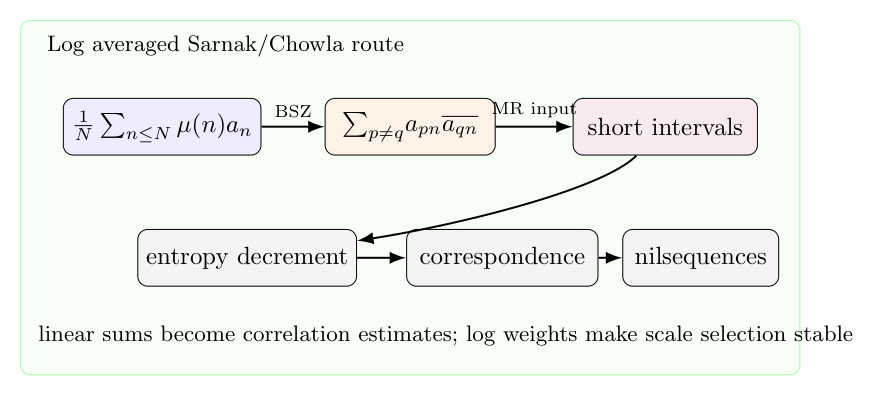
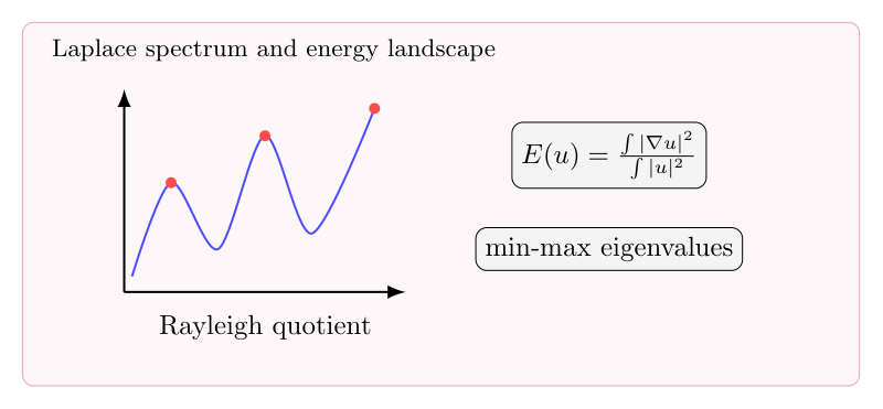

 arrive minimum?
 to be localized on small set.
 the Shwarz space, we begin with a intuition (not very rigorous) calculate:


 in
in  of level set
  in the whole space, this is of course a exponential sum.
 along one direction in frequency space, in fact we could say the inverse, i.e. it could not decay very fast.
 ,
,  is a ellipsoid.
 . It is said, for
  or
or  , so we have,
 ,
,  .
. but not the standard inner product
  ? How to understand the choice?
  .
.
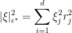
 related to
  .
.
 ,
,  , then it is not possible for
  .
. . Then,
 case is trivial by Paserval identity, which said on
  , fourier transform is a isometry,
  . For general case, integral by part, and use trivial estimate,
 ,
,  , every direction, we have
 , define
  . then we have the following:

 and are both true. then we use our favourite way to use Cauchy-Schwarz, the difficulty is we can not use a integral by part argument directly, even after restrict ourselves with monotonic radical symmetry inequality and by a rearrangement inequality argument, it seems reasonable due to rearrangement decreasing the kinetic energy as said in Lieb’s book. But even work with monotonic one, then one involve with some complicated form, try to use Fubini theorem to rechange the order of integral try to say something, it is possible to work out by this way but I do not know how to do. There is some calculate under this way,
 , the reasonable calculate is following,
 , Then
 … I do not know.
 we lose two cone very near
  , we need use the extra thing to make up them. May be effective argument come from some geometric inequality.
 are of finite measure, can there be a nonzero
  and
and  ? Some argument is folowing: Observe that:
 then
then  . So we have, at least
  . Some dirty calculate show:
 ,
,

 . So if
  then we can canculate we can not have
  in the original question.
 , so in all case. We have the following quatitative theorem:
 finite measure in
 .
.


 , then every thing become a discretization one, and the change could been argue as a approximation way. What happen then, we have a naive picture in mind which is:

 is very small, then use the argument
  could be given presicely by this way, but I do not care about it.
  .
. an suppose that
  satisfies,
 then
then
 as
as  .
. satisfies the following “thinkness” condition: there exists
  such that
 is arbitrary but fixed. Assume that
  . Then
 depends only on
  and
and  .
. be a polynomial, Then, for all
  , there exists
  such that
  in a distribution sence.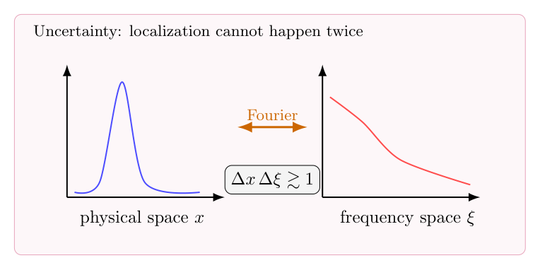


 is a non-degenerate closed
  form.
form. . we consider the gradient flow with
  as
as  . And we wish the gradient flow have a addition structure on itself then we could consider what is the Brunn-Minkowski inequality in this setting, the condition is a group structure on the space of level set
  , i.e.
 in
in  , if the induced gradient flow is amenable, then this is somewhat similar with the one dimension case, I wish if we could do something for the single function
  , then we can say something for the several functions involved case.
  measurale set in
 “>
“> ,
, 
 measurable set,
  ,
,  , and
, and  , and
, and
 algebra.
  .
.  . \newpage

 , one in finite field
  .
.  are finite set,we have,


 , then
 .
. , and make the additive energy
  decreasing. after induction with this transform and the transform from a tuple to the minimum additive energy by translation, the additive energy decreasing and decreasing then arrive the global minimum. But it is easy to conclude in this case one of
  , and
, and  are finite sets,
 , consider they be very thin line.
 ,
,  . So they have the trend tending to make the “boundary” campatible with “area”. Two thin line in the same direction is exactly the worst case, which is just a equal condition of 1-dimension case.
 is bounded by some constant. But this is also not the suitable set for our inequality, I explain how to capture the information of the G-H coverage.
 . We give the definition of
  discretization of
  ,
,  is the
  instead of
  depending on iff
  , where
  is a given number only rely on
 .
. rigorous meaning campatible with
  is the cube center at
  if it is in
  is lipchitz. So you will have some locolization property, said, at every fix discretization scale
  is morally known so the number of cubes in
  which is the subspace of
  dimensional hausdorff measure of
  . So at least,
 . In fact we a in the situation with Accumulation of wood to make the product have smallest volume. Not to optimized the tuples
  but fix one of it, said
  , the convex of the functional
  on convex set.
 .
. , there is a subspace
  with codimension 1 divide
  such that
 .
. different directions in
  , then easy to proof every line
  and a point
  on
on  , such that

 is a convex function on
 to optimized
  small. It is the same as make
  small when fix
  and
and  . Due to

![\displaystyle \Leftrightarrow 1\geq [\frac{\Pi a_i}{\Pi(a_i+b_i)}]^{\frac{1}{d}}+[\frac{\Pi a_i}{\Pi(a_i+b_i)}]^{\frac{1}{d}} \ \ \ \ \ (16)](https://s0.wp.com/latex.php?latex=%5Cdisplaystyle+%5CLeftrightarrow+1%5Cgeq+%5B%5Cfrac%7B%5CPi+a_i%7D%7B%5CPi%28a_i%2Bb_i%29%7D%5D%5E%7B%5Cfrac%7B1%7D%7Bd%7D%7D%2B%5B%5Cfrac%7B%5CPi+a_i%7D%7B%5CPi%28a_i%2Bb_i%29%7D%5D%5E%7B%5Cfrac%7B1%7D%7Bd%7D%7D+%5C+%5C+%5C+%5C+%5C+%2816%29&bg=ffffff&fg=000000&s=0&c=20201002)
![\displaystyle \begin{array}{rcl} \mu(A+B)^{\frac{1}{d}} & = & [\int_{{\mathbb R}}(\int_{{\mathbb R}^{d-1}}\chi_{A+B}(\xi_1,...,\xi_{n-1})d\xi_1...d\xi_{n-1} )d\xi_n]^{\frac{1}{d}}\\ & \sim & \frac{1}{\mu(A_n)}\int_{{\mathbb R}}(\int_{{\mathbb R}^{d-1}}\chi_{A+B}(\xi_1,...,\xi_{n-1})d\xi_1...d\xi_{n-1})^{\frac{1}{d-1}}d\xi_n\\ &\overset{induction \ on \ d} \geq & \frac{1}{\mu(A_n)}(\mu^{\frac{1}{d-1}}(A(\xi_n))+\mu^{\frac{1}{d-1}}(B(\xi_n)))d\xi \\ &\overset{A-G \ inequality} \geq & \mu^{\frac{1}{d}}(A)+\mu^{\frac{1}{d}}(B). \end{array}](https://s0.wp.com/latex.php?latex=%5Cdisplaystyle+%5Cbegin%7Barray%7D%7Brcl%7D+%5Cmu%28A%2BB%29%5E%7B%5Cfrac%7B1%7D%7Bd%7D%7D+%26+%3D+%26+%5B%5Cint_%7B%7B%5Cmathbb+R%7D%7D%28%5Cint_%7B%7B%5Cmathbb+R%7D%5E%7Bd-1%7D%7D%5Cchi_%7BA%2BB%7D%28%5Cxi_1%2C...%2C%5Cxi_%7Bn-1%7D%29d%5Cxi_1...d%5Cxi_%7Bn-1%7D+%29d%5Cxi_n%5D%5E%7B%5Cfrac%7B1%7D%7Bd%7D%7D%5C%5C+%26+%5Csim+%26+%5Cfrac%7B1%7D%7B%5Cmu%28A_n%29%7D%5Cint_%7B%7B%5Cmathbb+R%7D%7D%28%5Cint_%7B%7B%5Cmathbb+R%7D%5E%7Bd-1%7D%7D%5Cchi_%7BA%2BB%7D%28%5Cxi_1%2C...%2C%5Cxi_%7Bn-1%7D%29d%5Cxi_1...d%5Cxi_%7Bn-1%7D%29%5E%7B%5Cfrac%7B1%7D%7Bd-1%7D%7Dd%5Cxi_n%5C%5C+%26%5Coverset%7Binduction+%5C+on+%5C+d%7D+%5Cgeq+%26+%5Cfrac%7B1%7D%7B%5Cmu%28A_n%29%7D%28%5Cmu%5E%7B%5Cfrac%7B1%7D%7Bd-1%7D%7D%28A%28%5Cxi_n%29%29%2B%5Cmu%5E%7B%5Cfrac%7B1%7D%7Bd-1%7D%7D%28B%28%5Cxi_n%29%29%29d%5Cxi+%5C%5C+%26%5Coverset%7BA-G+%5C+inequality%7D+%5Cgeq+%26+%5Cmu%5E%7B%5Cfrac%7B1%7D%7Bd%7D%7D%28A%29%2B%5Cmu%5E%7B%5Cfrac%7B1%7D%7Bd%7D%7D%28B%29.+%5Cend%7Barray%7D+&bg=ffffff&fg=000000&s=0&c=20201002)
 such that it is a equality, by the equal condition of Minkowski inequality, in fact this is morally inverse of Minkowski inequality. The second reason in general case why the second inequality is true is due to a rescaling argument, change
  , by the rescaling argument we conclude if there is a such inequality, the index of it must be the case.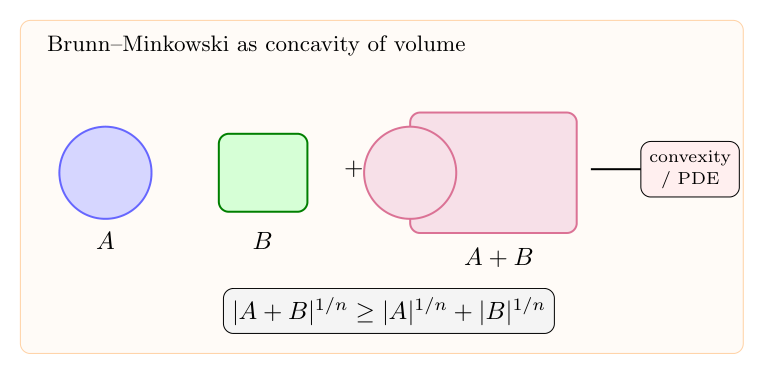

 could be represented by a multiplication operator on the Fourier transform side. translation is the meaning,
  is a translation.
 , then
 will consititue a dense set in
 when
when  is a bounded function, thanks to Parevel theorem. When
 , there is two approach, heat kernel approximation approach and discretization.
 ?
?
 , namely
  , so we need some decay condition on
  , why this, just consider integral by part for
  . The rigorozaton of this intuition inspirit us to the definition of symbol calss.
 is in symbol class
  iff,
iff,
 is multi-indece.
 , essentially the “characteristic polynomial” of the operator.
 , this kernel representation makes
  theory introduce in previous note is therefore applicable.
 and the Lipschitz space
  .
.
 is assume to be real, symmetric, positive definite and smooth in
  . Understanding
  , such that,
 .
.  is a error term which have good control. To do this, fix an arbituary point
  , freeze the operator
  at
at 

 vanish near the origin,

 is actually a smoothing operator, because it is given by convolution with a fixed test function. It should be seasonable when
  is well approximated by
  , it is actually the case, define
  , i.e.
 , where the error operator
  and is said to be of order
  of
of  function of
  and satisfies the differential inequality:
 ,
,  .
. 
 pointwise,
  ,
,  in
in 
 and take
  , if
, if  .
.  in the sense:
 ,
,


 denotes
  . Thus the pesudo-differential operator
  initially defined as a mapping from
  to itself
  such that,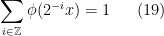
 , there is only two of
  such that
  , and we can choose
  to be radical and
  .
.  .
. Then the operator
  and by dual.
  satisfy, for any multi-index
  ,
,
 . Then, for any
  , there is a constant
  such that,

 are multi indeces. Then we consider dyadic decomposition, the is a function
  . then
  cpt,
cpt,  . So
. So  , we have,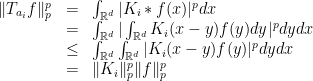
 have good decay estimate, thanks to
  , this estimate is deduce morally along the same ingredient of “station phase”, it is come from a argument combine “counting point” argument and a rescaling argument. So,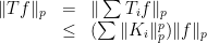
 , ending the proof.
 to
to  .
.
 .
.
 are symbols belonging to
  and
and  respectively. Then there is a symbol
  so that:


 .
.

 , so
, so

 in that variable, and allows us to rewrite
 , i.e.
 , due to
 and it is definitely the case, we get the theorem.
  , where
 .passage to the limit as
  will then give us our desired result.
 .
. . Then, we can express
  as
as
 , that,
 , this representation extends to all
  for almost every
  . More generally, we have,

 to itself, for
  .
.  if
if  and the partial derivatives
  , taken in the sense of distribution, belong to
  . The norm in
 , then
  , whenever
  .
.  to
to  , whenever
  .
.  . Then, as operator from
  to itself, the
  have norms that satisfy
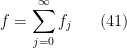
 , for all
  , where
  is the smallest integer
  .
. , the argument prove
  ,
,  , gives the required estimate for the
  .
. gives an isomorphism from
  , is continuous from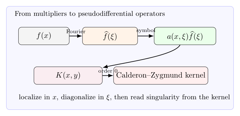
 .
. be a vector field, at once we have a vector field, we could consider the associated flow of it,
 along the vector field.
 . One the other hand, due to the locally existence theorem of ODE, if the regularity of
  is enough, then the solution exist and is uniqueness.
  or more convenient
  . We call
  the flow map or the exponential map generated by
  for all
  .
. for all
  .
. , the mapping
  is a diffeomorphism with
 . In local coordinate we have
  ,
,  express position of particle,
  express momentum of particle.
 in
in 
 matrix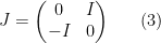
 .
. ,
, 
 and degenerate, i.e. if
  for all
  , then
  .
. ,
,  .
. , by basic linear algebra everything follows.
 , map
, map

 is called the symplectic form.
 , i.e.,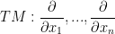

 , roughly we have
  , this is of course not true, but morally true. Now let us give the definition of symplectic manifold and the relationship of Hamiltonian mechanics.
 where
where 
 is symplectic, and
  is differentiable, the hamiltonian vector field of
  on
on 
 coordinate
  and the symplectic form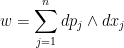
 is differentiable, then the integral curves of

 is a trajectory of the Hamiltonian flow of
 .
. , due to we have
  . So
. So  we have:
 . Then we have,
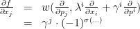
 such that
  ,
,  is given by
 ![\displaystyle \begin{array}{rcl} m\overset{\cdot\cdot}x & = & m(\overset{\cdot} {\frac{\partial f}{\partial p}})\\ & = & m\frac{\partial}{\partial t}(\frac{\partial f}{\partial p})\\ & = & m\frac{\partial}{\partial p}[\frac{\partial}{\partial t}(\frac{\|p\|^2}{m}+V(x))]\\ & = & m\frac{\partial }{\partial p}(\frac{2p\overset{\cdot}p}{m}+\frac{\partial V(x)}{\partial x}\cdot \frac{\partial f}{\partial p}) , due\ to \ -\frac{\partial f}{\partial x}=-\frac{\partial V(x)}{\partial x}.\\ & = & m\frac{\partial }{\partial p}(\frac{2p(-\frac{f}{\partial x})}{m}+\frac{\partial V(x)}{\partial x}\cdot \frac{\partial f}{\partial p})\\ & = &-\frac{\partial V(x)}{\partial x} \end{array}](https://s0.wp.com/latex.php?latex=%5Cdisplaystyle+%5Cbegin%7Barray%7D%7Brcl%7D+m%5Coverset%7B%5Ccdot%5Ccdot%7Dx+%26+%3D+%26+m%28%5Coverset%7B%5Ccdot%7D+%7B%5Cfrac%7B%5Cpartial+f%7D%7B%5Cpartial+p%7D%7D%29%5C%5C+%26+%3D+%26+m%5Cfrac%7B%5Cpartial%7D%7B%5Cpartial+t%7D%28%5Cfrac%7B%5Cpartial+f%7D%7B%5Cpartial+p%7D%29%5C%5C+%26+%3D+%26+m%5Cfrac%7B%5Cpartial%7D%7B%5Cpartial+p%7D%5B%5Cfrac%7B%5Cpartial%7D%7B%5Cpartial+t%7D%28%5Cfrac%7B%5C%7Cp%5C%7C%5E2%7D%7Bm%7D%2BV%28x%29%29%5D%5C%5C+%26+%3D+%26+m%5Cfrac%7B%5Cpartial+%7D%7B%5Cpartial+p%7D%28%5Cfrac%7B2p%5Coverset%7B%5Ccdot%7Dp%7D%7Bm%7D%2B%5Cfrac%7B%5Cpartial+V%28x%29%7D%7B%5Cpartial+x%7D%5Ccdot+%5Cfrac%7B%5Cpartial+f%7D%7B%5Cpartial+p%7D%29+%2C+due%5C+to+%5C+-%5Cfrac%7B%5Cpartial+f%7D%7B%5Cpartial+x%7D%3D-%5Cfrac%7B%5Cpartial+V%28x%29%7D%7B%5Cpartial+x%7D.%5C%5C+%26+%3D+%26+m%5Cfrac%7B%5Cpartial+%7D%7B%5Cpartial+p%7D%28%5Cfrac%7B2p%28-%5Cfrac%7Bf%7D%7B%5Cpartial+x%7D%29%7D%7Bm%7D%2B%5Cfrac%7B%5Cpartial+V%28x%29%7D%7B%5Cpartial+x%7D%5Ccdot+%5Cfrac%7B%5Cpartial+f%7D%7B%5Cpartial+p%7D%29%5C%5C+%26+%3D+%26-%5Cfrac%7B%5Cpartial+V%28x%29%7D%7B%5Cpartial+x%7D+%5Cend%7Barray%7D+&bg=ffffff&fg=000000&s=0&c=20201002)
 .
.  , conservation of energy. In orther word,
  , so the Hamiltonian flow of
  .
. , we have,
 . In general case, i.e. coordinate free proof,
  . Use identity if lie derivative. The second thing is also easy to proof by look in a local canonical coordinate, involve the indentity of lie derivative.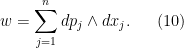
 is any smooth manifold, then its cotangent bundle
  has a natural symplectic structure.
  derive from
  , it is
  on
on  , the existence of Riemann metric involve a unit decomposition argument and bump function, I just recall it there. Now we move on, consider the relationship between
  .
.

 non-degenerate. This case in the lemma is a example to show that could be the case:
  be local coordinates on
  . Define a coordinate system
  by the condition:
 and therefore
  .
. be a smooth Riemann manifold and let
  be one half of the square of the Riemann norm, so that in local coordinate,

 is any smooth function on phase space (the symplectic manifold), then the rate of change of
 , the poisson bracket of
 , one has,
 .
.
 is a Lie algebra.

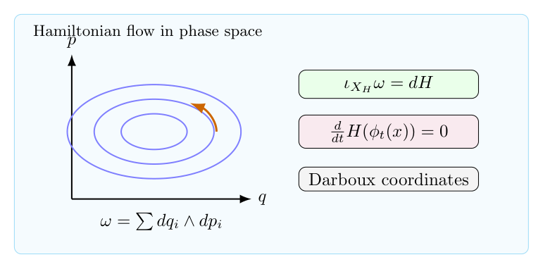
 , crossing each other and the is a set
  of crossing point. for technique reason, assume the position of lines are generic, i.e. no three of them intersect at one point. Then we could use 3 different colors to color
  case,
case,  is the number.
 , the single line by
  . The problem is try to find a tuple
  , where
  is a metric define on
  . such that the distortion of
  and the standard metric on
  in some sense? what could we say with this kind of